The theory of the “scatter degree” method (^{Guo, 2012})

The synthetic function is the linear function of greatest-type indicators (x₁, x₂,…, x_m):

(1)

where ω = (ω₁, ω₂ ... ω_m)^T is an m-dimensional pending positive vector.

Inserting the standard observed values (x_i1, x_i2,…, x_im) of evaluation object S_i into Eq. (1), Eq. (2) is acquired:

(2)

If and, Eq. (2) is converted to Eq. (3):

(3)

The variance of evaluation objects y = ω^Tx:

(4)

The principle of determining the weight coefficient of the “scatter degree” method is getting the linear function ω^Tx of index vector x and making the variance of the evaluated object’s values as high as possible; y = Aω is substituted into Eq. (4). When , the new formula is as follows:

(5)

where H = A^T A is a real symmetric matrix.

When ω is unlimited, formula (5) can be an arbitrarily large value. Here, ω^Tω = 1, and the maximum value of formula (5) is acquired. Namely, the value w is acquired to meet the constraints:

(6)

For formula (5), when w is standard feature vector of the largest eigenvalues of H, ω^T Hω achieves its maximum value. The weight coefficient vector (ω₁, ω₂, ... ω_m)^T is obtained by normalizing ω, and . The comprehensive values y_i of the evaluation object are obtained by using Eq. (2).

The improvement of the “scatter degree” method

The “scatter degree” method emphasizes that the method should highlight the differences among the evaluation objects as a whole, and it runs under the premise of the same importance of the evaluation target to every evaluation indicator. In fact, the degree of the importance is not same. The “function drive” theory provides the weighting coefficient r_j(j = 1,2, ..., m) of each indicator x_j. On this basis, each indicator is weighted by the following formula:

(7)

where x_ij are the standard observed values. The mean value and mean square deviation of x_ij^* are 0 and r_j², respectively. The weighting coefficient of weighted data {x_ij^*} is acquired by using the “scatter degree” method. Then, the comprehensive evaluation values can be obtained.

Analytic Hierarchy Process (^{Deng, Li, Zeng, Chen, & Zhao, 2012})

In this article, the Analytic Hierarchy Process (AHP) is used to confirm the weighting coefficients r_j of each indicator.

AHP was discovered by Satty while performing operational research in the 1970’s. The indicators are classified into several levels of objective, criterion, and index. This method is based on both quantitative and qualitative approaches.

The steps of AHP include building a hierarchical model, building a matrix of each level, performing a consistent check, and verifying the total arrangement of each hierarchy with a consistent check.

The evaluating data and its standards

Reference data was adopted from (^{Geng, 2012}). All the nine indicators are classified into positive and negative classes, and need to be standardized to remove the influence of inverse indices and different dimensions.

For the positive index:

(8)

For the negative index:

(9)

where and

Matrix A is calculated based on the raw data as well as Eqs. (8) and (9). The results shown as follows:

The application of vertical “scatter degree”

Symmetric matrix H is calculated by using the formula H = A^TA.

The maximal eigenvalue and eigenvector of matrix H′ is calculated by using MATLAB: λ_max (H) = 13.9332, ω(H) = (0.0768, 0.1124, 0.1280, 0.1287, 0.0980, 0.1144, 0.1391, 0.1436, 0.0591)^T.

The values of WECC in the years of 2005 and 2009 are calculated by plugging x_j (t_k) and w_j into Eq. (2).The results are shown in table 1.

Table 1 The results of WECC by two different methods. 

The application of AHP-Vertical “scatter degree”

Calculation of the weight using AHP

1. A system of evaluation is established according to the reference, which is as follows: 1) Level of objective: WECC; 2) Level of indicators: ratio of water resource to utilization and exploitation X₁, gross regional output per capita X₂, water consumption of GDP X₃, water consumption of industrial output X₄, discharged volume of wastewater of industrial output X₅, discharged chemical oxygen demand of industrial output X₆, repeated utilization rate of industrial wastewater X₇, attainment rate of the industrial wastewater X₈, daily water consumption per capita X₉.

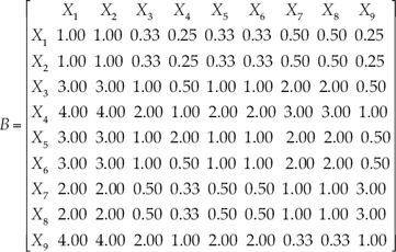
2. The weight of the index: The relative importance of all indicators was determined with reference to the literature. Then, matrix B is acquired as follows:

• Then, the weight of the indicator is obtained by using MATLAB: λ_max = 9.886, r = (0.043, 0.043, 0.127, 0.217, 0.127, 0.127, 0.092, 0.092, 0.133)^T.

1. Consistency check: 1) consistency index: , where n is the number of indicators, and CI = 0.11075; 2) consistency ratio: , where RI is the mean random consistency index, and when n = 9, RI = 1.46. So, CR = 0.07586 < 0.10, and the judgment matrix is consistent.

The WECC of AHP-Vertical “scatter degree”. The matrix X′ is acquired using Eq. (7).

A symmetric matrix H′ is derived from the formula: H′ = X′^TX′

The maximal eigenvalue and eigenvector of matrix H′ is calculated using MATLAB: λ_max′(H′) = 22.22, ω′(H′) = (0.0260, 0.0442, 0.1490, 0.2570, 0.1046, 0.1322, 0.1066, 0.1177, 0.0627)^T.

The values of WECC in the years of 2005 and 2009 were calculated by putting x_j(t_k) and w_j′ into Eq. (2). The results are shown in table 1.

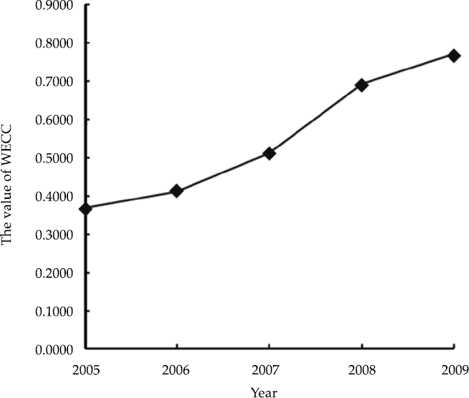
From the table and figures, it is clear that the results of the evaluation are basically consistent.

Figure 1 Water environmental carrying capacity of Shanxi Province spots (vertical “scatter degree” method). 

Figure 2 Water environmental carrying capacity of Shanxi Province spots (AHP-vertical “scatter degree” method).