


 texto en
  Inglés (pdf)
 Artículo en XML
 Referencias del artículo
 Enviar artículo por email
 Citado por SciELO
  Similares en
SciELO
Similares en
SciELO 
 Permalink
INTRODUCTION
The Carangidae family is comprised of a great variety of fish species spanning 31 genera (Nelson 2006, Froese and Pauly 2023). These species are distributed in the tropical and subtropical waters of the Atlantic, Pacific, and Indian Oceans, and some are of high economic value and exploited by both artisanal and industrial fisheries. For example, the horse mackerel (Trachurus murphyi) fishery in the South Pacific Ocean is becoming one of the most important fisheries in the world (Gerlotto et al. 2012, Lucano-Ramírez et al. 2016). One of the most representative genera of the Carangidae family is Selene, which is composed of 8 species that are distributed in the tropical coastal waters of the Atlantic and Pacific Oceans (Froese and Pauly 2022).
In Ecuador, Selene peruviana (Guichenot, 1866), which is locally known as Carita, is an important resource for artisanal and industrial fisheries. Selene peruviana is found in pelagic and demersal habitats along the continental shelf and forms shoals near the bottom between 10-80 m depth (Martinez 2005). Considerable volumes of this species are caught with purse seines, trawls, and gillnets. For example, the Ecuadorian sardine purse-seine fleet caught 5,402.8 t of S. peruviana as bycatch in 2004. The amount of bycatch has decreased since then, with 2,680.49 t of bycatch caught in 2019 (IPIAP 2022). The meat of S. peruviana, like that of several members of the Carangidae family, is well valued in the market and widely consumed (Jiménez and Béarez 2004). The effects of the overexploitation of coastal fisheries are further exacerbated due to pollution, climate change, and urban development (Díaz et al. 2016) and are reflected in reductions in catch volumes, biodiversity, organism size, growth rates, reproductive capacity, abundance, and biomass (González et al. 2007).
Information on the sex ratio and changes in maturity phases that occur throughout the year is critical for fully understanding the biological characteristics of a population and required for comprehensive evaluations of fisheries stocks (Holden and Raitt 1975). These characteristics allow for the reproductive potential of exploited fish stocks to be determined (Williams 2007). At the regional level, little research has been conducted on the biology of S. peruviana. In Ecuador, information regarding the biology of this species is scarce. Therefore, the present study aims to fill this knowledge gap regarding the reproductive dynamics of S. peruviana through an analysis of the size at sexual maturity and reproductive cycle. Our results serve as a baseline for future research efforts and contribute valuable insights for the management of this important resource.
MATERIALS AND METHODS
Sampling locations
Selene peruviana sampling was conducted between January 2017 and December 2018. Specimens were collected from the catches of artisanal fishers using gillnets in the artisanal fishing harbor of Los Arenales (0°51ʹ02.93ʺ S, 80°32ʹ02.84ʺ W) and from the landings of the industrial fleet that operates with purse seine nets in the fishing port of Manta (0°57ʹ00.18ʺ S; 80°42ʹ32.98ʺ W; Fig. 1). The coasts of Ecuador exhibit marked environmental seasonality. The rainy or humid season occurs from January to May when an increase in the sea surface temperature (SST) is observed. The dry season occurs from July to November and is characterized by a decrease in SST, with June and December considered transition periods (Perugachi et al. 2014, Prado and Cajas 2016).

The specimens were transferred to the biology laboratory of the Facultad de Ciencias del Mar of the Universidad Laica “Eloy Alfaro” de Manabí. Morphometric measurements were taken of all specimens, and their organs were extracted. Total length (TL) was measured with a digital ichthyometer (precision of 1 mm). Total weight (Wt), gonad weight (Wg), and liver weight (Wl) were measured with a digital balance (precision of 0.01 g). Sex was determined by visually analyzing the gonads, and gonadal maturity was visually estimated from macroscopic characteristics using an empirical scale following the methodology of Holden and Raitt (1975), with modifications. The stages of gonad maturity were the following: stage I, (immature), stage II (maturing), stage III (mature or gravid stage), stage IV (spawning), and stage V (regeneration).
Length-weight relationship
To estimate the length-weight relationship, the following potential allometric equation was used (Ricker 1975, Froese 2006):
where Wt is the total weight of the species, a the intercept, TL is the total length, b is the slope that describes the type of growth, and ϵi is the multiplicative error of the i-th fish. To estimate a and b, the least squares method was used by linearizing equation (1) via logarithmic transformations of Wt and TL.
Estimation of size at sexual maturity
The length at sexual maturity (L50) was estimated from the accumulated frequencies of stages III, IV, and V using 6 sigmoid models (Table 1).
Table 1 Models used to estimate the size at sexual maturity (L50).
| Author | Model |
| Gompertz (1825) |
|
| Richards (1959) |
|
| Bakhayokho (1983) |
|
| King (1995) |
|
| White (2002) |
|
| Brewer & Griffiths (2005) |
|
Parameters: Pi is the proportion of mature individuals in each size range (Lt), L50 is the length at which 50% of individuals reach sexual maturity, θ and r, the rate of change, m and k, adjustment parameters, a and b intercept and slope, and α is the amplitude of the maturity ogive.
Model adjustments were made by minimizing the negative of the verisimilitude logarithm (-LN[L]; Neter et al. 1996) based on the probability of a binomial distribution. The best fit of the models was verified using the Akaike information criterion (AIC; Akaike 1973):
where k is the number of parameters to be estimated in the model and -LN[L] is the negative logarithm of verisimilitude. The model that offers the lowest AIC value (AICmin) is the one in which the least information is lost and the one that best fits the data. Akaike weights (Wi) were calculated to determine the best fit model among all candidates:
where ʌi is the difference between AIC and AICmin of each model.
Spawning season
The spawning season was determined by analyzing the temporal variation of the gonadosomatic index (GSI) to determine the period or periods with the greatest reproductive intensity during an annual cycle (Brown-Peterson et al. 2011). The variation of the GSI was analyzed along with the variation of the relative condition factor (Kn) and that of the hepatosomatic index (HSI; Le Cren 1951, Vazzoler 1996, Smylie et al. 2016, Wang et al. 2016):
where Wg, Wt, and Wl are the gonad weight, total weight of the fish, and liver weight; respectively; TL is the total length of the fish; and b is an allometric factor.
Statistical analyses
Normality and homoscedasticity of the data were evaluated with Shapiro-Wilks and Bartlett tests, respectively. Differences in the length distribution between sexes were compared using a Kolmogorov-Smirnov test. The monthly differences in the size of S. peruviana by sex, GSI, HSI, and Kn were evaluated by a one-way analysis of variance (ANOVA) and post-hoc Tukey-Kramer tests. When the data did not comply with the assumptions of normality and homoscedasticity, Kruskal-Wallis tests were employed. A comparison of the sex ratio with the expected ratio (M:F) of 1:1 was conducted with a Chi-square (χ 2) test. To evaluate the growth type, the allometric factor (b) was compared to a value of 3 using Student t-tests. Pearson correlations were used to evaluate the relationships of GSI values between sexes (Zar 2010). Statistical tests were performed in Statgraphics Centurion (StatPoint Technologies, Inc., Warrenton, VA, USA) and R (R Core Team 2020). Significance was determined with α = 0.05 (P < 0.05).
RESULTS
Size distribution
A total of 886 specimens were analyzed (400 in 2017 and 486 in 2018; Table 2). In the size frequency distribution for both sexes, the TL values ranged from 10.50 to 41.30 cm, with an average TL of 23.16 ± 3.81 cm. There was no significant difference in the general size of individuals between 2017 and 2018 (t Student, P > 0.05). Females and males exhibited average TL values of 22.97 ± 3.73 and 23.62 ± 3.79 cm, respectively (Fig. 2). The size frequency distributions differed significantly between sexes (K-S test = 2.03; P < 0.05).
Table 2 Monthly statistical summary of sizes for 2017 and 2018.
| 2017 | 2018 | |||||||
| Month | n | Average | Range | SD | n | Average | Range | SD |
| Jan | 9 | 17.06 | 15.50-18.00 | ± 0.82 | 32 | 22.83 | 18.20-27.30 | ± 2.51 |
| Feb | 41 | 26.40 | 17.30-39.50 | ± 4.62 | 21 | 27.70 | 21.20-35.50 | ± 4.65 |
| Mar | 26 | 22.29 | 18.50-25.00 | ± 1.75 | 35 | 22.70 | 18.10-27.90 | ± 2.82 |
| Apr | 31 | 20.95 | 18.70-26.20 | ± 1.59 | 15 | 21.95 | 19.90-23.30 | ± 1.025 |
| May | 67 | 24.31 | 18.00-40.80 | ± 4.11 | 42 | 21.55 | 10.50-27.00 | ± 2.86 |
| Jun | 56 | 22.60 | 17.20-29.90 | ± 2.37 | 134 | 22.15 | 17.00-30.10 | ± 2.91 |
| Jul | 63 | 22.51 | 19.40-34.80 | ± 2.24 | 75 | 22.16 | 19.00-28.50 | ± 1.65 |
| Aug | 36 | 26.80 | 22.90-30.50 | ± 2.20 | 20 | 23.68 | 17.00-32.80 | ± 4.95 |
| Sep | 20 | 21.30 | 16.60-23.90 | ± 1.61 | 24 | 26.58 | 15.00-37.50 | ± 6.14 |
| Oct | 11 | 20.66 | 12.40-23.50 | ± 2.95 | 24 | 26.79 | 18.00-35.90 | ± 5.87 |
| Nov | 31 | 23.70 | 19.50-38.70 | ± 3.52 | 27 | 22.89 | 17.30-30.00 | ± 4.13 |
| Dec | 9 | 21.25 | 20.00-22.30 | ± 0.79 | 37 | 23.36 | 18.70-41.30 | ± 3.92 |
| Total | 400 | 23.43 | 12.40-40.80 | ± 3.69 | 486 | 22.99 | 10.50-41.30 | ± 3.96 |

Length-weight relationship
The potential model for all captured organisms was Wt = 0.0361TL2.63 with a coefficient of determination (r 2) of 0.89 (Fig. 3). The allometric factors (b) of females and males were 2.62 and 2.49, respectively, which were significantly less than 3. A significant difference between sexes with respect to the isometric parameter was found (Student t-test = 12.16, P < 0.05). Therefore, growth was considered to be negatively allometric for both sexes (Table 3).
Table 3 Total number of individuals, maximum and minimum sizes, and parameters of the length-weight relationship of Selene peruviana.
| Sex | N | Min. | Max. | Average | SD | a | b | r2 | P |
| Male | 353 | 17.00 | 40.80 | 23.62 | 3.79 | 0.057 | 2.49 | 0.86 | <0.05 |
| Female | 503 | 16.60 | 41.30 | 22.97 | 3.73 | 0.038 | 2.62 | 0.89 | <0.05 |
| Combined sexes | 886 | 10.50 | 41.30 | 23.16 | 3.81 | 0.037 | 2.63 | 0.89 | <0.05 |

Sex ratio
Of the 886 specimens analyzed, 353 were males and 503 were females, and sex could not be identified in 30 individuals. This resulted in a sex ratio (M:F) of 0.7:1.0, which was significantly different from the expected value of 1:1 (χ 2 = 26.28; P < 0.05).
Size at sexual maturity
The TL of the smallest mature specimen was 17.00 cm for both sexes. The maturity curves were calculated for males, females (Fig. 4), and sexes combined with the 6 previously described models. The highest L50 value was obtained with Richard’s model (31.12 cm TL, IC95% ± 0.87) for females, while the lowest L50 was obtained with the Gompertz model (20.59 cm TL, IC95% ± 0.97) for males. The Bakhayokho, King, and White models, allowed for the average length at sexual maturity of S. peruviana to be determined, with values of 22.61 cm TL (IC95% ± 0.98), 23.86 cm TL (IC95% ± 0.91), and 23.27 cm TL (IC95% ± 0.67) for males, females, and both sexes, respectively (Table 4).
Table 4 Multimodel adjustment and inference for Selene peruviana males, females, and sexes combined. AIC: Akaike Information Criterion, ʌi: difference between AIC and AICmin of each model; L50: length at sexual maturity; Wi%: weigth of each model.
| Model | Combined sexes | Female | Male | |||||||||
| L50 | AIC | ʌi | >Wi% | L50 | AIC | ʌi | Wi% | L50 | AIC | ʌi | Wi% | |
| Gompertz (1825) | 20.91 | 93.61 | 3.70 | 4.24 | 21.29 | 86.41 | 2.92 | 5.97 | 20.59 | 63.22 | 0.15 | 23.61 |
| Richards (1959) | 29.05 | 91.08 | 1.16 | 15.03 | 31.12 | 84.31 | 0.82 | 17.14 | 24.12 | 272.66 | 209.59 | 0.00 |
| Bakhayokho (1983) | 23.27 | 89.91 | 0.00 | 26.91 | 23.86 | 83.50 | 0.00 | 25.63 | 22.61 | 63.07 | 0.00 | 25.46 |
| King (2007) | 23.27 | 89.91 | 0.00 | 26.91 | 23.86 | 83.50 | 0.00 | 25.63 | 22.61 | 63.07 | 0.00 | 25.46 |
| White (2002) | 23.27 | 89.91 | 0.00 | 26.91 | 23.86 | 83.50 | 0.00 | 25.63 | 22.61 | 63.07 | 0.00 | 25.46 |
| Brouwer & Griffiths (2005) | 21.41 | 526.81 | 436.90 | 3.61 | 21.54 | 358.95 | 275.45 | 0.00 | 21.35 | 218.91 | 155.84 | 0.00 |
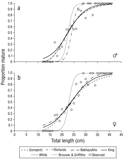
Figure 4 Sexual maturity curves with Gompertz (1825), Richards (1959), Bakhayokho (1983), King (2007), White (2002), and Brouwer and Griffiths (2005) model adjustments for Selene peruviana (a) males and (b) females.
Gonadal maturity stages
The monthly analysis of the gonadal maturity stages indicated that mature and immature individuals were present during most of the study period with variations in their respective percentages. In 2017 and 2018, the highest percentages of immature male specimens were observed in May, June, and July (Fig. 5a, b). The periods with the highest abundance of specimens with mature gonads were August-October 2017, February-April 2018, and August-September 2018 (Fig. 5a). Selene peruviana females exhibited a similar pattern to that of males, with the highest percentages of specimens with immature gonads present in April-June 2017 (Fig. 5c) and June-July 2018 (Fig. 5d). The highest percentages of specimens with mature and spawning gonads were observed in February and March of both years (Fig. 5c, d).

Reproductive cycle
The monthly values of the GSI exhibited significant differences during 2017 (H = 136.93, P < 0.05), with the highest values observed during the rainy season in February and March and the lowest values observed during the dry season in May-August, with a slight increase in September. The HSI showed significant differences (H = 50.44, P < 0.05) and values that exhibited a similar trend to those of the GSI, while the Kn demonstrated small variations throughout 2017 (H = 174.03, P < 0.05; Fig. 6a). In 2018, S. peruviana exhibited a similar pattern in GSI values, with the highest peaks observed in February and March and the lowest values observed in June and July (H = 100.40, P < 0.05). The HSI values were significantly different among study months (H = 107.74, P < 0.05) and exhibited a similar trend to those of the GSI (Fig. 6b), while the Kn exhibited significant differences (H = 28.04, P < 0.05) among study months with slight variations when compared to those of the GSI in 2018 (Fig. 6b).
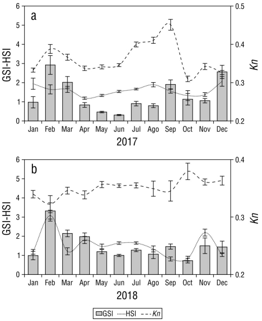
Figure 6 Monthly variation of the gonadosomatic index (GSI), hepatosomatic index (HSI), and relative condition factor (Kn) for sexes combined of Selene peruviana in (a) 2017 and (b) 2018.
The results of the Pearson correlation analysis indicated that no statistically significant correlations were present between the GSI and HSI (r = 0.35, P > 0.05) or between the GSI and Kn (r = 0.21, P > 0.05).
DISCUSSION
In the present study, the size range of S. peruviana differed from those reported by Tapia-García (1997), Tripp-Valdez et al. (2012), and Salazar-Céspedes et al. (2015). These differences may be due to the fishing gears used to collect specimens. In those studies, the samples were collected during oceanographic campaigns that employed trawls (1 3/4” mesh) during the shrimp fishing season. However, the size range observed in the present study was similar to those reported by Llanos et al. (2005) and Vera (2007), which can be attributed to the specimens in those studies being collected from commercial fishing campaigns in the Tumbes region in northern Peru. Due to the proximity of this region to Ecuador, the environmental conditions of these areas are similar as are the fishing gears (Table 5).
Table 5 Size, reproduction, and growth parameters of Selene peruviana reported in different studies.
| Species | Average size (cm TL) | Range (cm TL) | Size maturity (combined, cm TL) | Size maturity (males, cm TL) | Size maturity (female, cm TL) | b | Sex ratio (M:F) | Site | Reference | Country |
| Selene peruviana | 4.70-26.00 | Gulf of Tehuantepec, Mexico | Tapia-García (1997) | Mexico | ||||||
| Selene peruviana | 8.50-26.50 | Gulf of California | Tripp-Valdez et al. (2012) | Mexico | ||||||
| Selene peruviana | 17.80 | 14.00-23.00 | Tumbes Peru region | Salazar et al. (2015) | Peru | |||||
| Selene peruviana | 19.50 | 13.00-34.00 | 1.2:1.00 | Tumbes region | Llanos et al. (2005) | Peru | ||||
| Selene peruviana | 11.00-35.00 | 0.97:1.00 | Tumbes region | Vera (2007) | Peru | |||||
| Selene peruviana | 4.50-27.00 | 2.74 | East Coast of the mouth of the Gulf of California | Nieto-Navarro (2010) | Mexico | |||||
| Selene setapinnis | 9.74 | 2.90-21.70 | 2.79 | Sao Paulo, South East Brazil | Muto et al. (2000) | Brazil | ||||
| Selene vomer | 4.45 | 2.20-24.30 | 2.74 | |||||||
| Selene brownii | 2.84 | Gulf of Mexico | Farias-Tafolla et al. (2015) | Mexico | ||||||
| Selene vomer | 2.44 | |||||||||
| Selene dorsalis | 19.09 | 21.29 | 3.03 | 1.00:0.97 | Côte d’Ivoire | Arra et al. (2018) | Africa | |||
| Selene setapinnis | 1.08:1.00 | Gulf of Paria and the Orinoco River Delta | Molinet et al. (2008) | Venezuela | ||||||
| Selene setapinnis | 23.10 | 14.00-40.30 | 23.70 | Margarita Island | Tagliafico et al. (2012) | Venezuela | ||||
| Selene setapinnis | 21.50 | 20.50 | South East region of Brazil | Bastos et al. (2015) | Brazil |
Negative allometric growth was observed in S. peruviana, which was similar to that reported by Nieto-Navarro (2010) in Selene setapinnis and by Muto et al. (2000) for Selene vomer in Sao Paulo, southeastern Brazil. Farias-Tafolla et al. (2015) also reported negative allometric growth for Selene brownii and S. vomer in the Gulf of Mexico. These similarities among results can be attributed to Selene species having rectangular bodies that are highly laterally compressed, which makes Selene species morphologically unique (Reed et al. 2001) when compared to those of the other 31 genera of the Carangidae family that show fusiform morphologies (Jacobina et al. 2013). Thus, the type of growth exhibited by Selene species is likely determined by body shape, as this species increases in length more than weight while growing (Table 5).
The sex ratio of each species is highly variable (Claro 1994). The sex ratio found for S. peruviana was different from what was reported by Llanos et al. (2005), who found a sex ratio (M:F) of 1.20:1.00 for the same species. Similarly, Arra et al. (2018) reported a sex ratio of 1.03:1.00 for Selene dorsalis on the Ivory Coast of West Africa, while Molinet et al. (2008) reported a sex ratio of 1.08:1.00 for S. setapinnis between the Gulf of Paria and the Orinoco River Delta. In the present study, the number of females was larger than that of males, which can be attributed to the spatiotemporal segregation of females that approach the coast during the breeding season or to differences in factors such as longevity and mortality (Sylla et al. 2016). Moe (1969) considered that intense and sustained fishing pressure likely reduces the transition rate, thus increasing the reproductive potential of the population by increasing the number of females. However, in the present study, no significant differences were observed between the sizes of S. peruviana males and females, thus fishing pressure is unlikely to affect the sex ratio (Table 5).
In fishes, the onset of sexual maturity is more related to length than to the age of the individual (Saborido-Rey 2008). To estimate L50, the data should be distributed throughout the curve, from the tipping point to the asymptote (Birch 1999). However, this condition is often not met in exploited stocks due to the selectivity of fishing gears (Trippel and Harvey 1991). Currently, models adjusted by the verisimilitude method are widely used in fisheries research, and multimodel inference is useful for estimating a global model (Hernández-Covarrubias et al. 2013). Based on the AIC, the Bakhayokho, King, and White models offered the best fit to the data, thus these models were used for the overall estimation of L50.
Given that there are no records of the size at sexual maturity for S. peruviana in Ecuador, a temporal analysis of the influence of fishing pressure on the size at sexual maturity for this fisheries resource cannot be performed. However, in the present study, the size at sexual maturity was similar to the average size of capture, which could indicate that S. peruviana is currently at the limit of its optimal size of capture. In the future, this could result in instability with regard to the recruitment of new individuals to the population (Ochoa-Ubilla et al. 2016).
The size at sexual maturity can be compared to those of other Selene species. Our results are similar to those reported by Tagliafico et al. (2012) for S. setapinnis in the southern Caribbean Sea. It is noteworthy that the L50 of S. peruviana males was lower than that of females, which was also reported by Arra et al. (2018) for S. dorsalis on the Ivory Coast but different from what was reported by Bastos et al. (2015) for S. setapinnis in southeastern Brazil, who observed that the L50 of males was higher than that of females. The oceanographic conditions between the Pacific and Atlantic Oceans are different, and this variation in the size at sexual maturity can be observed among species in the same region and in the same species among different environments (Saborido-Rey 2008). A greater size at sexual maturity of females has been reported by other authors who have attributed this to energy expenditure during maturation, which is typical of tropical species (Lucano-Ramírez et al. 2016) (Table 5).
High GSI values are associated with advanced stages of gonadal maturation (Grier and Uribe-Aranzábal 2009). Likewise, variations in liver weight are associated with the allocation of energy for different life processes (McBride et al. 2015). In the present study, mature specimens were found during most of the study months, which indicated that S. peruviana exhibited a long reproductive period, grouping this species into the category of “income breeders” (McBride et al. 2015). The variation in GSI of S. peruviana was similar to the one described by Llanos et al. (2005), who reported decreasing GSI values from May to August (fall and winter in Peru or the dry season in Ecuador) in the same species. Tapia-García (1997) established that S. peruviana in the Gulf of Tehuantepec of Mexico exhibits a reproductive period from February to November (with a peak between March and May), which differs from what was found in the present study, as the reproductive period began in September with maximum peaks observed in February and March. The same author stated that both maturation and spawning in females and males are synchronous, which was also observed in both sexes in the present study. This could be attributed to S. peruviana forming large shoals, which are characteristic of Carangidae species (ARAP 2011). Long reproductive periods are characteristic of tropical species with short life cycles, as these allow tropical species to withstand environmental variation (Kaiser 1973, Tapia et al. 1997, Perera-García 2008) and environmental transition periods. In this study, greater variation was observed during the transition from the rainy to dry season. This may be the result of food availability during this period, which is an important factor for reproduction (Zapata et al. 1999, Acevedo et al. 2007).
In some fish species, the GSI values are inversely related to Kn and HSI (González and Oyarzún 2002, Plua-Santana 2020). In the present study, this relationship was only observed in September 2018 with the GSI and Kn. The increase in reproductive activity during the rainy season can be attributed to increasing sea temperatures that extend the reproductive cycle due to increases in primary productivity and food availability. In contrast, during the dry season, sea temperatures drop, and reproductive activity decreases. In this study, this was evident in the decline in the proportion of mature stages during this period. The similar pattern of variation observed in GSI, HIS, and Kn could indicate a reproductive strategy in which the species does not use the energy reserves stored in the liver during the gonadal maturation process. Instead, the energy required for egg and sperm formation may stem from the food available during reproductive periods (Acevedo et al. 2007, Zamora-Mendoza 2020) without influencing body condition or lipid accumulation during vitellogenesis.

