


 nueva página del texto (beta)
 Inglés (pdf)
 Artículo en XML
 Referencias del artículo
 Enviar artículo por email
 Citado por SciELO
  Similares en
SciELO
Similares en
SciELO 
 Permalink
1. Introduction
Anthony P. Thirlwall (1941 - 2023) was a revolutionary Keynesian economist1, he was very influential among economists2. He grounded the basis to develop an economic growth model in which the demand is the key to the working of the economies. In contrast with the supply side growth models in which inputs availability led to economic growth, Thirlwall (1979) showed that regardless of the inputs availability, the dynamic trade balance equilibrium is the main constraint to the growth rate of the economies, which can be relaxed through the increase of the growth rate of exports and the industrialization of the economies to decrease the income elasticity of demand for imports.
The aim of this paper is to show that the current industrialization processes, such as the Mexican one, focused on being a part of the global value chains, are not a sustainable way to improve a growth rate consistent with a constant trade balance as a percentage of GDP. This kind of industrialization does not generate domestic linkages with the rest of the domestic productive manufacturing sectors, and even worse, it induces stagnation or even a reduction of the domestic markets. On the contrary, the industrialization processes, such as the one follow by China, which generates domestic productive links, domestic industries producing goods to substitute imports and dynamic domestic markets complementing the performance of the export sectors are more sustainable.
Empirically, we apply an extended model (Vázquez Muñoz, 2018), which incorporates the capital accumulation as a determinant of the growth rate consistent with a constant trade balance as a percentage of GDP to explain the economic growth rate of China (during 1971 - 2022) and Mexico (for the 1961 - 2022 period). We also use three subperiods to compare some specific differences related to exports growth rates and capital accumulation regimes.
The study is organized as follows: Section 2 contains a literature review, with Thirlwall’s Law (Thirlwall, 1979), the exports super-multiplier effect (McCombie, 1985) and Thirlwall’s Law incorporating capital accumulation (Vázquez Muñoz, 2018). Section 3 presents the specific methodology to estimate the net capital stocks and the economic capacities for China and Mexico and the methodology used to estimate their import demand equations. Section 4 shows the results and discussion derived there from and, finally, our conclusions are presented in Section 5.
2. Literature review
Thirlwall’s law can be derived assuming an initial trade balance equilibrium:
where X is the exports level measured in domestic output, θ is the real exchange rate and M is the imports level measured in foreign output. Thirlwall (1979) assumes the real exchange rate is given and equal to one3. Therefore, the dynamic trade balance equilibrium is given by:
where x is the growth rate of exports and m is the growth rate ofc imports. The exports level is a function of the foreign income level:
where Y * is the foreign income level and ψ * is the income elasticity of demand for exports. On the other hand, the imports level is a function of the domestic income level:
where Y is the domestic income level and ψ is the income elasticity of demand for imports. Therefore, the growth rate of exports is given by:
where g * is the growth rate of foreign income. While the growth rate of imports is given by:
where g is the growth rate of domestic income. Substituting equations (4) and (5) in equation (2) and solving for g we get the growth rate of domestic income consistent with a dynamic trade balance equilibrium:
where g tb is the growth rate of domestic income consistent with a dynamic trade balance equilibrium. Equation (7) has very important implications related with the growth rate behavior of the economies:
Regardless the inputs availability, the dynamic trade balance equilibrium imposes a restriction on the growth rate.
The relative growth rate of the domestic economy with respect to that of the foreign economy is related to the international trade specialization of the economies. The economies specialized in manufacturing exports exhibit a lower income elasticity of demand for imports than the economies specialized in primary exports. When Thirlwall (1979) was published, there was a clear division between the international trade specialization of developed economies (manufacturing) and developing economies (primary goods). So, developing economies are condemned to exhibit a lower growth rate than developed economies4.
If the low growth rate economies want to accelerate their economic growth, they should implement industrialization processes to reduce their income elasticity of demand for imports.
Now, given that the numerator of equation (7) is the growth rate of exports (equation (5)), we can re-express equation (7) as:
Equations (7) and (8) are known as the strong and weak versions of Thirlwall’s Law5 respectively. Since the publication of the Thirlwall’s Law, it attracted a great deal of attention, there have been a huge number of theoretical and empirical papers discussing it6.
As indicated, in 1979 there was a clear division between the international trade specialization of developed and developing countries. However, during the last decades there has been a restructuring of the production process around the world. International trade is currently characterized by global value chains, which implies a distribution of the whole productive processes around of different countries; capital-intensive processes remain in developed economies whereas labor-intensive processes were relocated to developing economies. So, the essential Thirlwall’s idea has not changed but currently we should qualify his recommendation emphasizing that the economies should promote industrialization processes involving higher income demand elasticities for exports and lower income demand elasticities for imports (see Rodrik, 2018)7.
Another point related to the Thirlwall’s Law is McCombie’s exports super-multiplier. According to McCombie (1985), exports are the only component of the aggregate demand which can produce a domestic income level increase and at the same time a trade balance improvement; in contrast, the rest of the aggregate demand components contribute to a domestic income level increase but at a trade balance worsening cost. Suppose a simple Keynesian model:
where C is the domestic consumption level, I is the domestic investment level, G is the domestic government expenditure level, c is the marginal propensity to consume and m is the marginal propensity to import; all variables with a horizontal line above are autonomous aggregate demand components. Equation (9) shows the internal equilibrium, the equality between the aggregate demand and the aggregate supply. Then, the domestic equilibrium income level is given by:
where
Now, using equations (13) and (14), the trade balance is equal to:
where XN is the trade balance. Therefore, an increase in autonomous aggregate demand implies a trade balance worsening, except for the case of the exports level:
On the other hand, using equations (13) and (14), the equilibrium trade balance is given by:
therefore, the domestic income level consistent with equilibrium trade balance is given by:
where Y tb is the domestic income level consistent with equilibrium trade balance. But, in fact, there is nothing assuring the equality between Y E and Y tb . McCombie (1985) maintains that the components of autonomous aggregate demand can be used to equalize Y E and Y tb . Specifically, we can consider the autonomous government expenditure, so Y E and Y tb will be equal if:
Therefore, the autonomous government expenditure for which Y E and Y tb are equal is given by:
where
Implicitly, McCombie (1985) assumes a low-income elasticity of demand for imports and the existence of a domestic productive structure capable of meeting the higher domestic demand. So, the domestic market and, specially, the existence of domestic productive chains are very important for economic growth. If there are domestic productive chains and, also, a domestic industry capable of producing goods to substitute imports, then the exports super-multiplier effect would be stronger8.
According to Vázquez Muñoz (2018), capital accumulation can be incorporated in Thirlwall’s model to consider the importance of domestic productive chains and the domestic market. The extended model considers an alternative specification for the imports demand level as follows9:
where F is a positive constant, KB is the gross capital stock, D is the domestic demand for domestic goods, EC is the economic capacity10, and ψ K , ψ D , ψ X are the gross capital, domestic income generated through the domestic goods demand and exports elasticities of demand for imports respectively.
EC is a function of the net capital stock:
where H is a positive constant, and
where d is the growth rate of internal demand for domestic goods and ec is the growth rate of economic capacity. Now, assuming that the growth rate of exports is given and equal to x 0 , substituting x 0 and equation (26) in equation (2) and solving for d, we get:
where d tb is the growth rate of internal demand for domestic goods consistent with a dynamic trade balance equilibrium. The first term of the numerator of equation (27) shows the importance of exports in the promotion of domestic productive activities; a lower value indicates a lack of productive linkages with domestic sectors; the third term shows the domestic capacity to produce goods to substitute imports and the second term stands for the requirements of imported capital goods for production. So, we can get the growth rate consistent with a dynamic trade balance equilibrium as follows:
where g tb is the growth rate consistent with a dynamic trade balance equilibrium and λ and (1-λ) are the internal demand for domestic goods and the exports as a percentage of domestic output, respectively.
3. Methodology
Next, we use econometric methodology to estimate equations (25) and (26); then we obtain the internal demand for domestic goods and GDP growth rates consistent with a dynamic trade balance equilibrium for China (1971 - 2022) and Mexico (1961 - 2022)11.
As a first step, to compute economic capacity we estimate China’s and Mexico’s net capital stocks using the Perpetual Inventory Method (Berleman and Wesselhöft, 2014). The net capital stock can be calculated in the following way:
where subscript t is a time index and δ is the depreciation rate. Solving equation (29) for the growth rate of net capital stock obtains:
Now, assuming that the net capital stock
Then, using equation (31) we can elaborate the net capital stocks series whilst the gross capital stock is calculated as:
Next, following Shaikh (2016), we compute China’s and Mexico’s economic capacity estimating the following equation:
where ln is the natural logarithm operator; β i (i = 0, 1) are the parameters to be estimated, KS is the net capital stock adjusted by the relative Gross Fixed Capital Formation and GDP deflators, β 1 is the economic capacity elasticity with respect to net capital stock and u Yt is an error term. Our null hypothesis is that β 1 is strictly higher than zero.
Once equation (33) is estimated, economic capacity is calculated as:
Then, we estimate the import demand function with the following specification:
where β i (i = 3, 4, 5, 6) are the parameters to be estimated, β 4 , β 5 , and β 6 , are the gross capital stock, the internal demand for domestic goods and the exports elasticities of demand for imports, respectively, and u Mt is an error term. Our null hypotheses are: β 4 and β 6 are higher or equal to zero, whilst β 5 is strictly higher than zero.
Equations (33) and (35) are estimated by the Bound Test Approach cointegration methodology (Pesaran, et. al. 2001) for two reasons: 1) we are estimating a theoretical long-run growth rate, and 2) this approach is pertinent irrespective of whether the underlying regressors are purely I(0), purely I(1), mutually cointegrated or any combination of these characteristics. This is, definitely, a considerable advantage given the low power of the unit root test and the relatively small size of our data for each country.
Once the elasticities of demand for imports are estimated, we get the growth rate of internal demand for domestic goods consistent with a constant trade balance as a percentage of GDP substituting them in the following equation12:
Finally, the growth rate consistent with a constant trade balance as a percentage of GDP is calculated through equation (28).
4. Results and discussion
The Chinese economy has exhibited a growth rate higher than the Mexican economy during the last decades. Specifically, as it can be seen in Graph 1 and Table 1, considering the periods 1971 - 2022 for China and 1961 - 2022 for Mexico, the former exhibited an average annual growth rate of 8.58% whilst for the latter that average is equal to 3.58%. However, if we just consider the subperiod 1961 - 1981 (Mexico’s high growth rate experience), the average for China (1971 - 1981) was 6.18% whilst for Mexico it was equal to 6.87%. So, although very slightly, the Mexican economy grew at a rate higher than the Chinese economy. In contrast, during the years following the external debt crisis (1982 - 1988), China’s growth rate rose to 11.46% whilst Mexico suffered stagnation with a growth rate equal to 0.02%. Finally, during Mexico’s trade liberalization subperiod (1989 - 2022) based on the Washington Consensus (Williamson, 1990), the Chinese economy exhibited an average annual growth rate equal to 8.77% whilst the Mexican economy grew at 2.27%.
If we consider aggregated demand components during the whole periods, the average annual growth rate of internal demand for domestic goods was equal to 8.18% for China and 2.73% for Mexico; on the other hand, considering their respective average annual growth rate of exports, China (13.53%) outpaced Mexico (7.94%). Therefore, the differential growth rate between China and Mexico is more proportional to their differential growth rate of internal demand for domestic goods than to that of their growth rate of exports. The average growth rate of internal demand for domestic goods for China was equal to 5.72% from 1971 to 1981 and 6.65% for Mexico in 1961 - 1981; in contrast, the average annual growth rate of exports for China was equal to 17.92% whereas for Mexico it was equal to 11.07%. Therefore, again, during this subperiod the differential growth rate is more proportional to the differential growth rate of internal demand for domestic goods than to the differential growth rate of exports. During the 1982 - 1988 subperiod, the average annual growth rate of internal demand for domestic goods for China was equal to 11.32% and equal to -0.87% for Mexico. In contrast, the average annual growth rate of exports for China was equal to 13.61% whereas for Mexico it was equal to 8.26%. Once again, during this subperiod the differential growth rate is more proportional to the performance of the internal demand for domestic goods than to that corresponding to the differential growth rate of exports. Finally, from 1989 to 2022, China’s average annual growth rate of internal demand for domestic goods was equal to 8.33% and Mexico’s equal to 1.05%; whilst the former’s average annual growth rate of exports was equal to 12.10% and the latter’s 5.95%. So, in this last subperiod the greater relevance of the differential growth rate of internal demand for domestic goods vis-à-vis that of exports to explain overall differential economic growth is confirmed.
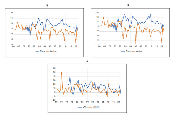
Notes: Series for China since 1971, whilst for Mexico since 1961. The internal demand for domestic goods was calculated as the difference between the GDP and exports.
Source: Author’s elaboration using data from the World Development Indicators database of the World Bank and from the National Accounts database of the United Nations.
Graph 1 GDP (g), internal demand for domestic goods (d) and exports (x) annual growth rates (%)
Table 1 GDP (g), internal demand for domestic goods (d) and exports (x) growth rates (annual averages)
| g | d | x | ||||
|---|---|---|---|---|---|---|
| China | Mexico | China | Mexico | China | Mexico | |
| 1971(61) - 2022 | 8.58% | 3.58% | 8.18% | 2.73% | 13.53% | 7.94% |
| 1971(61) - 1981 | 6.18% | 6.87% | 5.72% | 6.65% | 17.92% | 11.07% |
| 1982 - 1988 | 11.46% | 0.02% | 11.32% | -0.87% | 13.61% | 8.26% |
| 1989 - 2022 | 8.77% | 2.27% | 8.33% | 1.05% | 12.10% | 5.95% |
Notes: Series for China since 1971, whilst for Mexico since 1961. The internal demand for domestic goods was calculated as the difference between the GDP and exports.
Source: Author’s elaboration using data from the World Development Indicators database of the World Bank and from the National Accounts database of the United Nations.
How can we explain the behavior of the annual growth rates of internal demand for domestic goods for China and Mexico? As indicated, capital accumulation is relevant to induce an export super-multiplier effect through the creation of domestic productive chains and the production of goods to substitute imports. First, we calculated China’s and Mexico’s net capital stocks following the Perpetual Inventory Method. We calculated the investment trend growth rate for China and Mexico, which was equal to 2.75% for the former and 15.77% for the latter13. Then, we calculate the net capital series using equations (31) and (29). In Graph 2 and Table 2 our results are shown along with both countries’ investment coefficients.
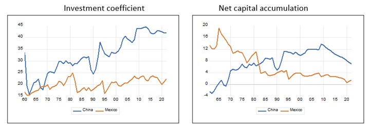
Source: Author’s elaboration using data from the World Development Indicators database of the World Bank, from the National Accounts database of the United Nations and from the Penn World Table 10.01 database.
Graph 2 Annual investment coefficient and net capital accumulation, 1960 - 2022 (%)
Table 2 Investment coefficient and net capital accumulation (annual averages)
| Investment coefficient | Net capital accumulation | |||
|---|---|---|---|---|
| China | Mexico | China | Mexico | |
| 1960 - 2022 | 32.43% | 20.18% | 7.65% | 3.62% |
| 1960 - 1981 | 24.24% | 19.43% | 3.19% | 6.19% |
| 1982 - 1988 | 30.63% | 18.34% | 8.23% | 3.83% |
| 1989 - 2022 | 37.85% | 21.02% | 10.28% | 1.99% |
Source: Author’s elaboration using data from the World Development Indicators database of the World Bank, from the National Accounts database of the United Nations and from the Penn World Table 10.01 database.
As shown in Graph 2 and Table 2, the Chinese investment coefficient was a bit higher than 50% than the Mexican one for the whole period (1960 - 2022). Moreover, in each subperiod of analysis the Chinese investment coefficient was higher and the lowest difference, by far, was during the 1960 - 1981, when the Mexican growth rate was higher than the Chinese one. With respect to the net capital accumulation, the Chinese rate was higher than the Mexican rate during the whole period and during the 1982 - 1988 and the 1989 - 2022 subperiods. In contrast, during the 1961 - 1981 subperiod, the Mexican net capital accumulation was almost 100% higher.
Next, we calculate the Chinese and Mexican economic capacities estimating equation (33). Previously, we present the unit root test for lnY and ln(KS) in Table 3.
Table 3 Unit root test for lnY and ln(KS), 1960 - 2022
| lnY | ADF test | PP test | lnKS | ADF test | PP test |
|---|---|---|---|---|---|
| China | -2.04 | -5.19* | China | -7.49* | -6.89* |
| Mexico | -1.74 | -1.75 | Mexico | -1.28 | -1.27 |
| d(lnY) | ADF test | PP test | d(lnKS) | ADF test | PP test |
| China | -8.70* | -9.73* | China | -3.28** | -3.03** |
| Mexico | -5.52* | -5.51* | Mexico | -4.39* | -6.30* |
Significance levels * p < 0.01, ** p < 0.05.
Notes: d(() stands for the first difference operator; all level tests were done assuming the existence of trend and intercept whilst all first difference tests were done assuming the existence of intercept. The lags numbers used for the ADF tests were chosen according to the Schwarz information criterion, whereas the number of Bandwidth used for the PP tests were chosen according to the Newey-West criterion.
Source: Author’s elaboration using data from the World Development Indicators database of the World Bank, from the National Accounts database of the United Nations and from the Penn World Table 10.01 database.
As shown in Table 3, lnY and ln(KS) for the Chinese case could be considered as a stationary series, whilst in the case of Mexico both series can be considered as integrated of order one. The results of our estimations of equation (33) by the ARDL cointegration methodology for China and Mexico are shown in Table 4.
Table 4 Estimation of the Economic Capacity
| Dependent variable | lnY | ||
|---|---|---|---|
| Period | 1960 - 2022 | ||
| China | Mexico | ||
| Constant | -4.46** | Constant | 11.19* |
| (1.79) | (0.38) | ||
| D9722 | 10.06* | ln(KS) | 0.62* |
| (2.55) | (0.01) | ||
| ln(KS) | 1.12* | D8222(ln(KS) | -0.01* |
| (0.06) | (0.001) | ||
| D9722(ln(KS) | -0.33* | ||
| (0.08) | |||
| Model type | Restricted constant and no trend | ||
| ARDL model | (3, 3, 2, 3) | (3, 4, 3) | |
| F-statistic | 8.28* | 21.80* | |
| Adjustment coefficient | |||
| ut-1 | -0.17* | -0.41* | |
| (0.06) | (0.04) | ||
| Jarque-Bera normality test | 1.94 | 0.38 | |
| LM test (F-statistic) | 2.61 | 1.64 | |
| White test (F-statistic) | 1.21 | 0.57 | |
| Ramsey RESET test (t-statistic, one fitted term) | 1.66 | 0.13 | |
Significance levels * p < 0.01, ** p<0.05.
Note: Standard errors in parentheses. White tests do not include cross terms. We use some dummy and composed dummy variables to capture structural breaks; DXXYY stands for a dummy variable with value equal to one from 19XX to 20YY and zero otherwise. ARDL model indicates the lags numbers of the dependent and independent variables. A complete report of the estimations, including the fixed regressors used in each case, is available on request from the author.
Source: Author’s elaboration using data from the World Development Indicators database of the World Bank, from the National Accounts database of the United Nations and from the Penn World Table 10.01 database.
As shown in Table 4, our estimations are robust; moreover, in both cases there was a structural break indicating a decrease of the economic capacity elasticity with respect to the net capital stock, in the case of China since 1997 and in the case of Mexico since 1982.
Once we got the economic capacity series for China and Mexico, we estimate the import demand equation (22). In Table 5 we present the unit root series test for each of the variables used.
Table 5 Unit root test for lnM and ln(KB), lnD-ln(CE) and ln(X)-ln(CE)
| lnM | ln(KB) | lnD-ln(CE) | lnX-ln(CE) | |||||
|---|---|---|---|---|---|---|---|---|
| ADF test | PP test | ADF test | PP test | ADF test | PP test | ADF test | PP test | |
| China | -1.92 | -0.93 | -2.16 | -2.77 | -2.81 | -3.18*** | -0.80 | -0.15 |
| Mexico | -3.37*** | -2.41 | -4.46* | -4.15* | -2.33 | -2.33 | -2.72 | -2.34 |
| d(lnM) | d(ln(KB)) | d(lnD-ln(CE)) | d(lnX-ln(CE)) | |||||
| ADF test | PP test | ADF test | PP test | ADF test | PP test | ADF test | PP test | |
| China | -5.92* | -5.24* | -2.76*** | -2.88*** | -5.88* | -5.88* | -4.72* | -4.70* |
| Mexico | -6.22* | -6.23* | -1.35 | -1.20 | -7.92* | -7.92* | -6.79* | -7.14* |
| ADFOBP test | ||||||||
| Mexico | -6.82* | |||||||
| (1981) | ||||||||
Significance levels * p < 0.01, ** p < 0.05, *** p < 0.10.
Notes: Series for China from 1970 to 2022 whereas series for Mexico from 1960 to 2022. ADFOBP is the Augmented Dickey Fuller test considering one break point test, break year in parentheses. d(() stands for the first difference operator; all level tests were done assuming the existence of trend and intercept whilst all first difference tests were done assuming the existence of intercept. The lags numbers used for the ADF tests were chosen according to the Schwarz information criterion, whereas the number of Bandwidth used for the PP tests were chosen according to the Newey-West criterion.
Source: Author’s elaboration using data from the World Development Indicators database of the World Bank, from the National Accounts database of the United Nations and from the Penn World Table 10.01 database.
According to our results, all series used for the estimation of the equation (35) are integrated of order one. The results of our estimations of equation (35) by the ARDL cointegration methodology for China and Mexico are shown in Table 6.
Table 6 Estimation of the Import Demand equation
| Dependent variable | lnM | ||
|---|---|---|---|
| 1970 - 2022 | 1960 - 2022 | ||
| China | Mexicoa | ||
| Constant | 5.06*** | Constant | 10.74* |
| (2.64) | (2.15) | ||
| D7075 | -0.23* | ln(KB) | 0.56* |
| (0.08) | (0.07) | ||
| ln(KB) | 0.81* | D8622(ln(KB) | 0.12* |
| (0.07) | (0.01) | ||
| ln(D)-ln(CE) | 2.43* | ln(D)-ln(CE) | 1.52* |
| (0.84) | (0.50) | ||
| ln(X)-ln(CE) | 0.98* | D8622(ln(X)-ln(CE) | 1.59* |
| (0.15) | (0.15) | ||
| Model type | Restricted constant and no trend | ||
| ARDL model | (4, 3, 2, 4, 2) | (2, 0, 0, 0, 0) | |
| F-statistic | 16.02* | 8.07* | |
| Adjustment coefficient | |||
| ut-1 | -0.35* | -0.47* | |
| (0.03) | (0.06) | ||
| Jarque-Bera normality test | 2.40 | 0.71 | |
| LM test (F-statistic) | 0.48 | 0.01 | |
| White test (F-statistic) | 0.45 | 7.36* | |
| Ramsey RESET test (t-statistic, one fitted term) | 0.76 | 0.97 | |
Significance levels * p < 0.01, ** p < 0.05, *** p < 0.10.
a Standard errors adjusted by the White procedure; White test includes cross terms.
Note: Standard errors in parentheses. We use some dummy and composed dummy variables to capture structural breaks; DXXYY stands for a dummy variable with value equal to one from 19XX to 19YY(20YY) and zero otherwise. ARDL model indicates the lags numbers of the dependent and independent variables. A complete report of the estimations, including the fixed regressors used in each case, is available on request from the author.
Source: Author’s elaboration using data from the World Development Indicators database of the World Bank, from the National Accounts database of the United Nations and from the Penn World Table 10.01 database.
As shown in Table 6, the gross capital elasticity of demand for imports is a bit higher in China than in Mexico; moreover, the domestic demand for domestic goods elasticity of demand for imports for China is higher than for Mexico, almost by one point; in contrast, whereas from 1961 to 1985 the exports elasticity of demand for imports was higher for China than for Mexico, from 1986 to 2022 it is the other way around. So, the Mexican liberalization strategy resulted in an export sector disconnected from the domestic economy.
The estimated internal demand for domestic goods and GDP annual growth rates consistent with a constant trade balance as a percentage of GDP are very similar to the actual ones for both economies (see Graph 3 and Table 7); in fact, the biggest differences observed in the Mexican case are for the 1989 - 2022 subperiod and, specially, for the 1982 - 1988 subperiod. Since the external debt crisis exhibited in 1982 until 1988, the Mexican growth rate could be equal to 6.34% but the economic policy was designed to depress the economic activity to get trade balances surpluses. On the other hand, during the liberalization subperiod (1989 - 2022) the growth rate consistent with a constant trade balance as a percentage of GDP has been so low (0.39%) that even although the actual annual growth rate has been low (2.27%), the Mexican economy has exhibited a cumulative trade balance deficits. Finally, it is worth noting that although the China’s average annual growth rate of exports has been higher during the whole period and during the subperiods than the Mexico’s, its gross capital contribution to the growth rate consistent with a constant trade balance as a percentage of GDP has been higher than its exports contribution, and the contrary is verified for the Mexican case, except during the liberalization period, for which the contribution of exports is negative and that of gross capital contribution is lower than one percentage point.
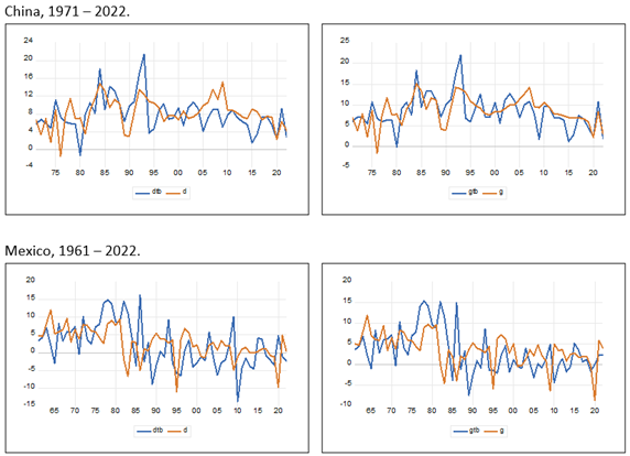
Source: Author’s elaboration using data from the World Development Indicators database of the World Bank, from the National Accounts database of the United Nations and from the Penn World Table 10.01 database.
Graph 3 Internal demand for domestic goods and GDP annual growth rates, observed and consistent with a constant trade balance as a percentage of GDP
Table 7 Internal demand for domestic goods and GDP growth rates, actual and consistent with a constant trade balance as a percentage of GDP; exports and gross capital accumulation contributions, observed and predicted GDP growth rate differential and variation of the trade balance as a percentage of GDP (annual averages)
| d | d tb | g | g tb | xc | (I/K)c | g-gtb | ∆xm | |
|---|---|---|---|---|---|---|---|---|
| China | ||||||||
| 1971 - 2022 | 8.18% | 7.89% | 8.58% | 8.43% | 2.37% | 6.06% | 0.15% | 0.09% |
| 1971 - 1981 | 5.72% | 6.03% | 6.18% | 6.47% | 0.58% | 5.89% | -0.30% | -0.03% |
| 1982 - 1988 | 11.32% | 11.89% | 11.46% | 12.00% | 0.87% | 11.13% | -0.54% | 0.39% |
| 1989 - 2022 | 8.33% | 7.76% | 8.77% | 8.33% | 3.26% | 5.07% | 0.44% | 0.07% |
| Mexico | ||||||||
| 1961 - 2022 | 2.73% | 2.16% | 3.58% | 3.19% | 2.25% | 0.94% | 0.39% | 0.04% |
| 1961 - 1981 | 6.65% | 6.45% | 6.87% | 6.66% | 6.10% | 0.56% | 0.21% | -0.02% |
| 1982 - 1988 | -0.87% | 6.11% | 0.02% | 6.34% | 4.39% | 1.94% | -6.32% | 1.34% |
| 1989 - 2022 | 1.05% | -1.30% | 2.27% | 0.39% | -0.57% | 0.96% | 1.88% | -0.18% |
Notes: xc is the exports contribution to the growth
rate consistent with a constant trade balance as a GDP percentage
and it was calculated as
Source: Author’s elaboration using data from the World Development Indicators database of the World Bank, from the National Accounts database of the United Nations and from the Penn World Table 10.01 database.
5. Conclusion
Thirlwall’s Law is a current and highly relevant idea for understanding the growth rate behavior of the economies. A. P. Thirlwall stresses the necessity of industrialization in developing countries to improve their growth rates. As Prebisch (1950), he saw the restructuring of the productive structure of the economies as a way to generate higher growth rates. From 1979, year of the publication of the Thirlwall's Law, there have been many contributions supporting, criticizing, empirically applying, and theoretically extending it; there is no doubt about the high importance of Thirlwall’s Law among economists.
When A. P. Thirlwall wrote his paper about the dynamic trade balance equilibrium constraint to economic growth rate in 1979, there was a clear division between developed and developing economies, the former specialized in manufacturing exports goods whereas the latter in primary exports goods. Currently, the global value chains modified the role of developed and developing countries in the international trade; some developing countries became manufacturing exporting countries; however, most of their production is focused on labor intensive processes, exhibiting a low-income elasticity of demand for exports and, on the other hand, they are not creating domestic productive chains nor a robust domestic market. Therefore, international trade benefits for them are not significant and, on the contrary, their specialization is contributing to the stagnation of activities oriented to the domestic market.
The contribution of the present paper is to show that exports could exhibit a low contribution to the growth rate consistent with a constant trade balance as a percentage of GDP if the export sector is not linked to the rest of domestic productive sectors. Moreover, capital accumulation is relevant if it induces domestic productive chains and the emergence of domestic industries producing goods to substitute imports. Industrialization processes do not have to be focused on the countries static comparative advantage, but on the generation of a domestic industry properly chaining most domestic subsectors.
Empirically, we show that although China’s exports growth rate has been higher than Mexico’s during the last decades, its most important contributor to the growth rate consistent with a constant trade balance as a percentage of GDP has been capital accumulation, whereas in the Mexican case, its more important contributor has been the exports. The Chinese industrialization process generated domestic chains among its domestic subsectors and the emergency of domestic industries producing goods to substitute imports. In contrast, the Mexican industrialization process was focused on specific labor-intensive activities not linked with the rest of the domestic industrial subsectors; its international trade liberalization resulted in the disappearance of many domestic industries that produced final goods.
It is worth nothing two results for the Mexican case: first, from 1989 to 2022, its growth rate consistent with a constant trade balance as a percentage of GDP is just 0.39%; the Mexican economy only can escape from stagnation through the accumulation of trade balance deficits, which, of course, is not a sustainable strategy; and second, during the same period (1989-2022) the exports growth rate is contributing in a negative way to the growth rate consistent with a constant trade balance as a percentage of GDP, this highlights the lack of domestic chains but also that the domestic market must be reduced ever more and more to maintain a sustainable trade balance deficit, which could have negative implications for key variables such as low wages, low government expenditure, high interest rates and, in general, the requirement to adopt contractionary economic policies.

