1. Introduction
One of the main abilities that unmanned vehicles should have is the capacity to estimate their relative position within an exploration environment. What is more, complex missions like resources detection and obstacle avoidance, require also that the vehicle be able to build a detailed map of its surroundings. A manner to acquire such knowledge is through the use of mapping methods, where a model of the nearby terrain is recovered from the measurements provided by onboard sensors. It’s well known in the literature that the problem of positioning and mapping are interconnected, and both have to be solved simultaneously (Grisetti et al., 2010). Systems that are capable of position estimation and mapping are known in the literature as Simultaneous localization and mapping (SLAM) (Cadena et al., 2016). There exist different kinds of sensors that can be utilized to accomplish the SLAM task (Lemus et al., 2014). A very interesting choice is the monocular camera. These kinds of sensors have, with the current state of technology, very large resolutions and also very high refresh rates.
There are many SLAM systems currently present in the literature that successfully use a monocular camera as the only sensor for resolving the SLAM problem. One example is LSD-SLAM (Engel et al., 2014), which uses an epipolar search approach together with a Kalman filter for estimating the depth of some of the pixels of a frame taken from a position of reference. The pixels that, due to lack of texture in the frame, cannot be estimated accurately are detected and discarded, and their depths are not estimated. With the depth of the pixels and the position of the reference frame, a local map is constructed. For the frames taken in nearby positions, the information obtained from their relative position within the local map is used to improve the reference frame pixels depth estimation. Another example is DSO (Engel et al., 2018), which takes an even more restrictive approach with the selection of pixels to be used for depth estimation. Only a very small percentage of the pixels in the frame are used for depth estimation. The resulting map is a very sparse one, but the results in localizations are outstanding. Other works like ORB-SLAM (Mur-Artal et al, 2015) use a pre-processing step on the captured frames, to identify the areas where robust depth estimation is more plausible. This pre-processing utilizes a salience detector to filter the zones of the frame that are not well posed for depth and pose estimation. All of these methods do not try to recover a detailed map of the surrounding terrain, focusing their attention on correct position estimation. Therefore, the usefulness of these methods in missions that require detailed knowledge of the surrounding terrain is questionable.
DTAM (Newcombe et al., 2011) tries to estimate depth in every pixel. A brute force plane sweeping approach (Hosni et al., 2013) in conjunction with a regularizer is used to accomplish this task. The system is still based on a pixel-wise epipolar search. And so, the estimation in areas in the frame where there is no texture is heavily regularized with the depth of nearby pixels, in order to recover somewhat correct depth estimations. REMODE (Pizzoli et al., 2014) uses an epipolar depth search together with a probabilistic measurement merging, again with a regularization at the end of the process. Zones in the frame where there is no texture must be, again, heavily regularized. The work of (Zienkiewicz et al., 2016) tries to estimate a mesh from the frames taken from a monocular camera. The system utilizes first a plane sweeping method similar to (Newcombe et al., 2011) to estimate the depth, and then this information is used to optimize every vertex of the mesh. The use of a pixel-wise estimation method makes again the zones without texture difficult to estimate and it requires the use of a depth regularizer.
It has been lately recognized in the literature that the depth smoothness hypothesis introduces a prior knowledge of the scene that many times is not accurate (Engel et al., 2018; Goodfellow et al., 2016). A better prior hypothesis on the depth of the scene is desirable. A surfel representation for the depth estimation could potentially resolve these issues. This would replace the depth smoothness prior with a more plausible piecewise planar depth prior, preserving strong discontinuities commonly found in man-made structures. Also, the representation of a part of the scene with the same parameters could avoid the need for a regularizer. Many works found in the literature have utilized surfels to represent the surface of the scene, but always using depth camera sensor like (Wang et al., 2019; Whelan et al., 2016; Yan et al., 2017).
This work presents a dense monocular SLAM system that does not utilize the depth smoothness prior. This method accomplishes the map estimation task by modeling the map, not as a group of independent points, but as a group of surfels. This takes advantage of the knowledge that the depth of most scenes can be modeled as a piecewise planar surface, instead of just a group of independent pixels. Every piecewise portion of the scene can be estimated with a surfel. This approach allows to directly restore robust and accurate pixel depths, even in zones where there is no good texture observation. Furthermore, this approach avoids the need for a regularization step. This way we can save on computational resources and, more importantly, it does not add a physically unlikely smoothness prior. New surfels can be initialized with the information of neighbor surfels. The entire system was written in the GLSL shading language, thus using the onboard GPU to achieve real-time. As far as the authors know, this is the first time this approach is used for monocular depth estimation. The method was tested on various data sets and the results show that both the depth and the surfels can be recovered correctly, demonstrating the potential of the method to reconstruct the scene with high quality.
2. Direct surfel optimization
In this section, we fully detail our depth estimation approach by direct surfel optimization. This section is structured as follows. First, in section 2.1, we explain which parameters are needed to describe the surfels. Then, in section 2.2, we explain how we obtain the inverse depth of the entire scene from the surfels set. Afterward, in section 2.3, we explain how we initialize the surfles’s parameters, before the optimization starts. In section 2.4 we present our surfel parameter optimization approach, using only the camera’s raw measurements (thus making this a direct method). Finally, in section 2.5, we explain how this surfel set is used to estimate the scene depth from another camera pose.
2.1. Surfel parameterization
Each surfel position p s and normal n s are defined relative to the pose P kf ∈ SE(3) of a reference frame F kf . The surfels have 3 free parameters, 2 belonging to the degrees of freedom of its normal n s , and the other given by the inverse depth id s of the ray r s going from the origin of the reference frame to p s , whose coordinates are given by
The radius of the surfel r is selected so that all surfels have the same frame-space area in the reference frame F kf , regardless of its normal or depth. This is done to guarantee the same quantity of pixel observation for every surfel, this way allowing to gather enough information for the Gauss-Newton estimation process.
Along with the aforementioned parameters, the last residual of each surfel and the time that the surfel was last seen and updated are stored for later use.
2.2. Inverse depth calculation
With the information provided by the estimated surfel parameters, the inverse depth id u of every pixel u belonging to the reference frame F kf can be obtained. Every u has a corresponding ray r u with coordinates
where K is the camera matrix, π() is the homogenizing function π([x,y,z]) = [x/z,y/z,1] and u ∈ R3 is a homogeneous pixel coordinate relative to Fkf. To be in the same plane, the point p s and p u = r u /id u must satisfy n s (p s −p u ) = 0, so id u is computed as
The inverse depth id u will be calculated relative to a surfel s when the distance between u and the coordinates of the surfel p s projected into the frame F kf , u s = π(Kp s ), is less than the radius r of the surfel s in screen space, that is
The GLSL shading language is utilized for the implementation of the system, so it allows the introduction of a depth buffer for occlusion removal. This means that, if several surfel project the same pixel screen location, only the pixels with the closest depth to the camera are selected.
During inverse depth computation, along with the depth information the index of the generating surfel sind is saved, for subsequent utilization as described below.
2.3. Surfel parameterization
To initialize the surfels, the reference frame F kf ’s inverse depth is computed. Clearly, in areas in the image where no surfel satisfies the equation 4, there will be no inverse depth measurement. These areas are identified as potential location to initialize a new surfel.
First, a search is carried out for an empty pixel u ns where a new surfel can be placed. This area must satisfy that there is no other inverse depth measurement nearby such that ∀Unn, ‖Uns −Unn‖> αr, where Unn is a non-empty pixel.
Then, all neighboring surfels are searched for. A neighbor surfel have to satisfy that a corresponding inverse depth measurement pixel us is nearby, with a distance of less than ‖Uns −Us‖< βr. The inverse depth for the new surfel is calculated as the mean of the estimated inverse depth, following equation 3 with respect to all nearby surfels s. The normal of the new surfel is initialized as the mean of all neighboring surfel’s normal.
Insofar as the real surface is globally plane, this type of initialization will give good results. This allows to initialize the surfel with the approximate correct surfel normal and depth, which allows to initialize the Gauss-Newton optimization, without the need to search for surfel initializing parameters.
2.4. Surfel optimization
The parameters of the surfels are estimated so that they minimize the cost function:
which is the commonly used sum of the Huber normed photometric error (Engel et al., 2018; Newcombe et al., 2011; Pizzoli et al., 2014) between the reference frame intensity I kf and every frame I fn in a group Ω of frames taken before I fn .
The coordinates u p of the pixel u as seen from the frame I fn can be calculated with
where
To recover the parameters of each surfel [n
s
,id
s
] that minimizes C([n
s
,id
s
]), a Levenber-Marquat (Engel et al., 2018) Gauss-Newton optimization
approach is implemented. The Jacobian
where
and
Furthermore,
As
Notice that even
2.5. Surfel reference frame change
A new reference frame
where
3. Implementation
The proposed system is implemented using the parallel computing capabilities of common GPUs, by utilizing OpenGL core 3.3. This way good performance is achieved without the need to have a high performance system capable of CUDA or OpenCL.
This depth estimation approach is integrated with the LSD-SLAM system (Engel et al., 2014), thus having position estimation and map management. It was found that this system is a good choice, because of its state of the art performance while being open-source and easy to expand upon.
3.1. System evaluation
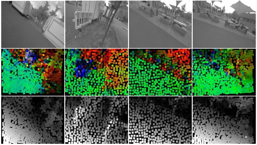
The system was evaluated in 3 benchmark datasets available in (TUM, Department of Informatics, 2017). These datasets depict 3 different scenes. The first dataset was taken on a foodcourt, with tables and benches in view. The street road present in the scene has a very smooth texture, so estimating its depth can be difficult. The second dataset was taken from inside a launch buffet, so the scene has many non-diffuse surfaces, such as the floor and doors. The last scene was taken walking around a machine building, so there are many open spaces and intricate structures. The dataset was obtained using a wide angle global shutter camera. The images are undistorted, and all camera calibration parameters are given by the dataset’s authors.
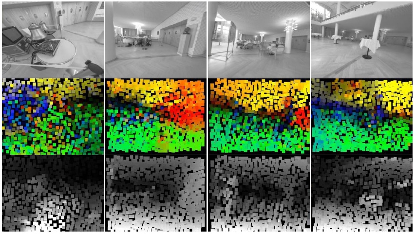
In the following sections, results show how the depth and the normal of the objects are recovered for different environments. The color codes present in the figures are as follows. For the normal estimations, blue represents vectors whose directions are facing to the right edge of the frame, and red represents vectors which are pointing to the right of the frame. Similarly, green represents vectors pointing up, and yellow are vectors pointing down. For the depth estimation figures, black represents a low inverse depth, and therefore high depth. Conversely, white represents high inverse depths, and so depths close to the camera focal point.
For the following evaluations, the camera image has a 640x480 resolution, and the surfel size was set to a radius of 10 pixels.
Foodcourt dataset: Results from the foodcourt dataset are shown in Fig. 1. It can be seen that the resulting depth is correctly recovered, even in the low texture sections of the street. The first column of Figure 1 depicts a backward moving movement. This means that the pixels in the lower part of the image are pixels just entering the frame, and so they have received very few observations. This highlights the usefulness of the surfel initialization scheme explained in section 2.3. The third column of Figure 1 depicts a forward movement, showing that both types of movements allow correct normal and depth estimations. In the second column it can be seen that the guarding fence, the food truck and the floor have correct depth and normal estimations. This part of the dataset is particularly challenging, because the guarding fence was seen a few frames ago from the opposite side, so its normals had the inverse direction. The same happens with the normals of the food truck.

Figure 1 Foodcourt dataset results. First column: raw frame. Second column: estimated normals. Third column: estimated depth.
Eccv dataset: This dataset is particularly challenging, because of the specularities present in almost all of the surfaces. The floor, the ceiling, and even some of the furniture present in the scene have this characteristic. The first column of Fig. 2 shows that the floor depth and normal were correctly estimated, even when there are specularities and blurriness. In the second, third and fourth columns of Fig. 2 it can be seen that the depth and normal of the ceiling were correctly recovered. The movement in the second row was backward, so all of the pixels in the lower part of the frame are new and with very few observations.

Figure 2 Eccv dataset results. First column: raw frame. Second column: estimated Normal. Third column: estimated depth.
Again this shows the usefulness of the surfel initialization.
Machine dataset: This dataset has the particularity that it was taken outside, and the sky is a very prominent part of most of the frames. As it was a cloudy day, the sky has texture, even when it is very smooth with a very low gradient. As can be seen in Fig. 3, the depth of the sky was correctly recovered, even with the conditions described before.
3.2. Usefulness of normal estimation
The usefulness of the joint depth and normal estimation was tested, by modifying
the Levenberg-Marquardt estimation algorithm described in 2.4. In equation 9,
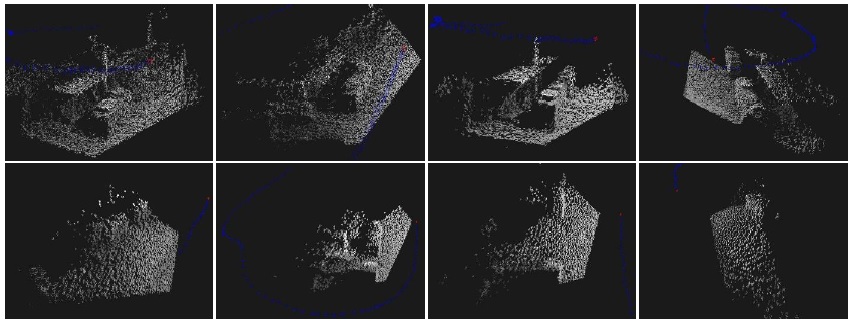
The resulting surface reconstruction of the foodcourt dataset with and without normal estimation can be seen in Fig. 4. The resulting scene reconstruction has a quality not present in the reconstruction made without normal estimation.

Figure 4 Detail of reconstruction, using a surfel radius of 5 pixels. First row: proposed method. The benches and tables present in the scene are easily recognizable, resulting from the correct surface normal estimation. Second row: without estimating surfels normals. This time the scene cannot be easily recognized, and artifacts caused by incorrect surfel normals are present.
3.3. Impact of surfel size selection
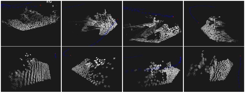
In this evaluation, the surfel radius was set to 12 pixels wide. Results of the scene reconstruction can be seen in Fig 5. The widening of the surfel causes a coarse reconstruction result, losing many details present on the scene. Nevertheless, the proposed approach can reconstruct the scene correctly, including the surfels on the floor and benches. Without using normal estimation the resulting reconstruction has a very poor quality, at the point of almost being unrecognizable, as seen in Fig 5.

Figure 5 Detail of reconstruction with a surfel radius of 12 pixels. The first row shows results with the present method, while the second row shows results without estimating the surfels normal. With the proposed method, even with such a coarse surfel reconstruction size, the benches and tables present in the scene can be still recognized, and the floor is correctly recovered. On the other hand, without estimating the surfels normal, the scene is almost completely unrecognizable, and there are heavy plane-depth related artifacts.
4. Conclusions
The approach described here can estimate a monocular dense depth map as a set of surfels, directly from the raw image pixels. As far as the authors know, this is the first time this approach is utilized for monocular depth estimation. This presents several advantages over methods more commonly found in the literature, that implement pixel depth estimation followed by a regularization schema. Firstly, there is no need for a computationally costly and physically unlikely depth regularization. Also, the information from the normal estimation can be used to initialize new neighboring surfels, thus being able to initialize the Gauss Newton optimization approach without the need to perform further computations.
The method was tested in several datasets, showing that the depth and surfels can be recovered correctly. The normal estimation allows for a more precise scene reconstruction, even when the surfel pixel radius is incremented considerably.
Most monocular depth estimation approaches present in the literature perform pixel wise depth estimation in conjunction with depth regularization methods. The results obtained in this paper suggest that more plausible depth priors can be utilized for scene reconstruction.
Since the proposed method has as objective fast robust dense depth estimation, unlike most of the methods currently present in the literature that aim just for sparse depth estimation, a proper comparison with the benchmark methods would only be possible in a real-time setting. Therefore, the next step aims to implement our and other benchmark methods on a mobile robot with an integrated GPU computer.


 nueva página del texto (beta)


