


 nueva página del texto (beta)
 Inglés (pdf)
 Artículo en XML
 Referencias del artículo
 Enviar artículo por email
 Citado por SciELO
  Similares en
SciELO
Similares en
SciELO 
 Permalink
1. Introduction
this study). Most of these methods are intrusive, expensive, complicated, and point measurement methods. Meaning if you are looking to measure wave parameters at a different location along the water surface or to obtain the spatial change in water surface elevation, a huge number of sensors or gauges should be used. These gauges must be calibrated with specific equipment to get the desired accuracy. Also, these gauges are in direct contact with the flow field means the flow field disturbance is frequently unavoidable (Hernández et al., 2018; Liu et al., 1982; Lee & Wang, 1984; Yao & Wu, 2005). Optical sensors (Blenkinsopp et al., 2012; Li et al., 1993; Payne et al., 2009), ultrasonic sensors (Blenkinsopp et al., 2010; Vousdoukas et al., 2014) have been used to evaluate the water surface elevation. To overcome the limitations of the intrusive methods, nonintrusive image-based techniques have been developed to obtain the water surface elevation (Douglas et al., 2020; Escudero et al., 2021; Hernández‑Fontes et al., 2020; Hernández et al., 2018; Iglesias et al., 2009; Yao & Wu, 2005).
Study (Siddiqui et al., 2001) used a PIV technique with a CCD video camera that was mounted above the water surface, and it is looking down at an angle of 34( from the horizontal axis to estimate the water surface elevation. The constant threshold value that was calculated based on the average grayscale value below the water surface was used to detect water surface elevation. In Hwung et al. (2009) water surface elevation obtained by using a CCD camera that was mounted above the water surface with three different angles from the horizontal axis. They detected water surface elevation using two detection algorithms, which were the hyperbolic tangent function (HTF) and threshold method (TM). In Mukto et al. (2007) a DPIV technique was used with a CCD camera that was mounted above the water surface, and it is looking down at an angle of 11( from the horizontal axis to estimate the water surface elevation. Water surface elevation was detected by the edge detection algorithm based on the variable threshold method. In Bonmarin et al. (1989) a visualization technique was used to perform a wave profile. This technique required a visible water surface under a given illumination, and this was done by using a thin sheet of light to illuminate fluorescein that was put in the flume tank. In their experiment the CCD video camera was placed in front of a flume tank to record the wave profile. Water surface elevation was detected by converting the digital image (signal) to a binary image (digital) that was done by applying an operator-adjustable threshold level. In Wang et al. (2012) integrated the modified plane-based camera calibration (MPCC) with an inexpensive internet web camera as the imaging device to measure water surface elevation. In Yao and Wu (2005) the DPIV technique was used with a CCD camera to detect water surface elevation. Wave profile was detected using a gradient vector flow active contour model (GVF) snake. In Erikson and Hanson (2005) a CCD video camera was used to measure wave profile. To form a visible video under a given illumination, the uniform light source was used to illuminate fluorescent green dye that was put inside the flume tank. Then they transferred the digital data from the camcorder to the computer using a high-speed interface. Surface water elevation was detected by employing the Matlab’s edge command (Robert’s edge detector) in the signal processing toolbox. In Zarruk (2005) particle image velocimetry (PIV) was used with a CCD camera to detect water surface elevation using the location of the maximum intensity gradient. The Bonferroni coefficient was used to detect the location of the maximum intensity gradient. In Viriyakijja and Chinnarasri (2015) two CCD video cameras were used and mounted perpendicular to the flume tank. They used canny edge detection to detect water surface elevation. They used a zero-up crossing method to obtain wave height and wave period. Then they solved dispersion relation with Hunt’s equation to obtain wavelength. Also, by using these methods relationship between time(frequency) and change in water surface elevation was produced, then wave height and period could be found by Rayleigh distribution or zero up crossing methods. The wavelength could be obtained by solving dispersion relation with one of the numerical methods that were explained later in this paper. Thus, significant errors could be found by using numerical methods to get wavelength. Up to the author's knowledge wavelength was evaluated indirectly by getting the value of wave height and frequency, and then using numerical methods to get wavelength. The current study was focused on getting the direct value of wavelength and eliminating the errors that may produce by solving dispersion relation theory by one of the numerical methods. All the above-mentioned literature compared their results with results obtained from conventional methods (capacitance wave gauges or pressure sensor) for verification. In this study, the PIV technique was used to capture the image for the water gravity waves at different frequencies. Then these images were analyzed by using the edge detection algorithm that was built using Matlab to get wavelength and wave height experimentally and these values are considered as the true value of wave measurements. Then, compared with the values obtained from the theoretical method (flap wavemaker transfer function theory) and conventional method (pressure measurement). Thus, the main objective of this study is to measure the performance of these three methods to measure the intermediate water gravity wavelength and wave height. While the wave period (frequency) is easy to get, as explained later, by using a digital photosensor tachometer, or can be considered as the time required for the 100-wave crests to pass a fixed point at 2 m far away from the wavemaker, using a stopwatch (Saincher & Banerjee, 2015)
2. Experimental setup and measurements
2.1. Experimental setup
This experiment focused on the intermediate water gravity waves

2.2. Wave parameter measurements
Mechanically driven wavemaker made of plexiglass hinged at the bottom of the flume tank with adjustable wave amplitude and wave frequency that produce sinusoidal wave motion. The electrical motor wave generator that was used to drive the Plexiglas flap wavemaker is composed of a ¼ HP, maximum 1725 RPM, 115 V, and 4.4 A. Electrical motor and a Plexiglas flap, see Figure 2.

Waves were generated by a flap-type bottom-hinged paddle mounted at one end of the tank, which travels down the trough and is employed to dissipate smoothly on the slope of the beach, or it can be called a wave absorber, as seen in Figure 1. The paddle (wavemaker) was driven by an electrical motor. Various paddle motion was achieved by varying the rotational speed of the electrical motor.
Three methods were used to obtain wave height, wavelength, and period. Firstly, Honeywell pressure sensors were mounted at the bottom of the wave tank at two different locations: one at 1 m from the wavemaker (PS1) and the other at 5 m from the wavemaker (PS2) to get a fully developed wave, as shown in Figure 1. Wave height and period were obtained from pressure reading, and then the linear wave theory equation was implemented, especially dispersion relation to getting wavelength. Secondly, analyzed PIV images to obtain the values of wave height and wavelength. Finally, by assuming that the frequency of the wavemaker is the same as wave frequency, then the dispersion relation could be used to get wavelength and then use the transfer function of the flap wavemaker (the relationship between wave height and the wave paddle stroke) to get wave height.
3. Mathematical modeling
3.1. Wave characteristics
Four parameters define characteristics of the gravity wave that are: height (H, m) or amplitude (a=H/2, m), length (L, m), period (T, sec) or angular wave frequency (

Wind waves are classified according to the ratio between still water depth and wavelength (h/L). Thus, wind waves are considered as deep-water waves when the still water depth is greater than half of the wavelength
3.2. Linear gravity wave theory
Linear gravity wave theory, also known as the Airy wave theory, is defined as the most straightforward theory used to obtain equations that provide the kinematic and dynamic properties for a two-dimensional small-amplitude surface gravity wave. The linear wave theory assumes that the ratio of the wave height to wavelength is less than 1/7, which means small wave steepness. The main assumptions for the linear wave theory are as follow:
1- Water is considered as a homogenous and incompressible fluid, and wavelength is greater than 3 cm so that the capillary effect can be neglected.
2- Flow is irrotational; that is no shear stress anywhere at the air-water interface or the bottom of the tank.
3- The bottom of the tank is not moving and is impermeable and horizontal, which means there is no energy transfer through the bottom.
4- The pressure along the air-water interface is constant; that means there is no effect of wind on the pressure difference between maximum at crest and minimum at the trough.
The most important assumption is the wave amplitude is small compared to the wave height and still water level.
3.2.1. Governing equations
1- Navier - stokes equation, as shown in Eq.1
Where
By ignoring the viscous force and expanding the above equation into two considered directions (x, z), the following two Euler equations are derived, respectively, as shown in Eq. 2 and 3:
2- Continuity equation, as shown in Eq. 4
Introduce the velocity potential function
Integrate the above equation on (x, z) directions, respectively; the following Eq. 7 and 8 are obtained:
As shown above, the two force equations are precisely the same, but the second equation includes gravity effects. Therefore, a single equation for the whole field was developed and is known as the Bernoulli equation for unsteady irrotational flow, as shown in Eq. 9.
The continuity equation is transformed to the Laplace equation as follows in Eq. 10:
Defined Boundary conditions as follows:
1. The kinematic boundary conditions at the bottom of the wave tank. Based on the previous assumption, we assumed the bottom of the wave tank is not moving, as shown in Eq. 11.
2. The boundary condition at the water-free surface
a- Kinematic boundary condition related to the vertical velocity at the water-free surface, as shown in Eq. 12.
b- Dynamic boundary condition related to the pressure at the water-free surface, as shown in Eq. 13
The boundary condition at free water surface must be linearized and reapplied at still water level
Velocity potential function
Wave surface profile
The dispersion relation is known as the relationship between the wave frequency and wavenumber at a given still water depth. It was derived by adding the two linearized boundary conditions at the free water surface (dynamic and kinematic) together, then applying velocity potential and differentiating. This yield Eq. 18.
3.3. Pressure under waves
Pressure under the still water level depends on two factors: hydrostatic pressure due to the depth of still water and the dynamic pressure caused by waves. The pressure at any water level can be obtained by applying the Bernoulli equation for unsteady irrotational flow, as shown in Eq. 19.
Since we are dealing with a linearized condition, the second-order term
The first term represents hydrostatic pressure, and the second term represents dynamic pressure (wave pressure). See Figure 4.

4. Methods of measuring wave heights
4.1. Based on the theory of flap wavemaker
There are many ways used to generate regular waves such as piston type, flap (hinged) type, or plunger-type (Dean & Dalrymple, 1991). In the present work, flap (Hinged) type was used to generate regular waves in the wave tank in the fluid dynamics lab at Western Michigan University. Wave paddle stroke is defined as the maximum stroke distance that can be traveled by flap wavemaker at the free water surface (S, cm). The stroke of the flap was adjusted from 5.43 cm at the still water level (17 cm) to 11.5 cm at the top of the wave tank (36 cm), see Figure 5. The flap was attached to the bottom of the wave tank by a hinge that allows the flap wave maker to move forward and backward with the rotation of the electrical motor, as was shown in Figure 2.

Wave frequency, wavelength, and wave height were controlled by adjusting the stroke of the flap wavemaker and the frequency of the electrical motor. A digital photosensor tachometer was used to measure the electrical motor frequency with an accuracy of ±0.05%. To use the theory of flap wavemaker, the frequency of the wave paddle should be the same as the frequency of the wave generated. Thus, wave frequency was also measured by the time required for the 100 wave crests to pass a fixed point at 2 m far away from the wavemaker, using a stopwatch. Many wave crests were selected as the period of waves was up to 0.958 sec. So, it’s obvious that human error in measurements would be reduced if the time taken for passage of the 100 wave crests through a specific point were measured as opposed to say, for example, the ten wave crests. Hence, the accuracy in measurements of wave period increase with the number of waves under consideration (Saincher & Banerjee, 2015). The result was very close, and the error between the two readings was between (0.048%, 0.035%, and zero), and that means the results could be used to apply the transfer function of the flap wavemaker, as follows in Eq.21, (Dean & Dalrymple, 1991):
To use the Eq. 21, it should have the value of wavelength first. So, in this method, dispersion theory was used to get wavelength then substituted back into transfer function to get wave height. Thus, the wavelength cannot be directly solved for a given set of wave periods (T) or still water depth(h) from dispersion theory. Therefore, to get the wavelength value, it should be found by iteration. In this study, four numerical methods were used to get wavelength, as explained later.
4.2. Based on pressure measurements
In this study, two Honeywell pressure sensors were used to measure wave height. They were placed one and five meters away from the flap wavemaker. These sensors should not be placed directly at the water medium; thus, these sensors were fixed outside the wave tank and connected with a clear plastic tube, and that tube was tied and fixed at the bottom of the wave tank. These pressure sensors are designed to provide the outcome reading for the pressure. That means the outcome readings must be calibrated to obtain the actual readings of the pressure then turned to wave height by using Rayleigh distribution and zero down crossing method. Firstly, the two Honeywell pressure sensors must be calibrated to connect the measured value and actual pressure reading. The calibration test was done twice for two Honeywell pressure sensors. The calibration test was done by placing the pressure sensor as mentioned above, then changing the depth of still water above the pressure sensor. In the meantime, measured value (outcome from the pressure sensor) was recorded and calculated with the corresponding value of the actual hydrostatic pressure, as follows in Eq. 22:
Where
Table 1 Hydrostatic pressure and corresponding outcome of pressure sensor at different still water depths.
| Still Water Depth(m) | Measured Value m v | Actual Hydrostatic Pressure (P, Pa) |
| 0.1725 | 0.00358579 | 1692.225 |
| 0.123 | 0.003499 | 1206.63 |
| 0.1 | 0.003402 | 981 |
| 0.07 | 0.003326 | 686.7 |
| 0.05 | 0.003320 | 490.5 |
| 0 | 0.00320 | 0 |
The information in the table above allows us to draw a relation between measured and actual reading to get a calibration correlation, as shown in Figure 6.

As seen in Figure 6, the correlation coefficient
Where
Maximum Pressure reading was measured at the crest at
Minimum Pressure reading was measured at the Trough at
Wave height is the difference between the maximum and minimum wave surface elevation

Thus, Wave Height can be evaluated from Eq. 26.
As seen in the above equation, wave height is the function of wavenumber,
that was solved by using the Newton Raphson numerical method. Two Matlab codes were built to avoid manual calculation and get an accurate value of wave height, as seen in the following Figures 8, 9, and 10, and were evaluated at three different wave frequencies. The significant wave height
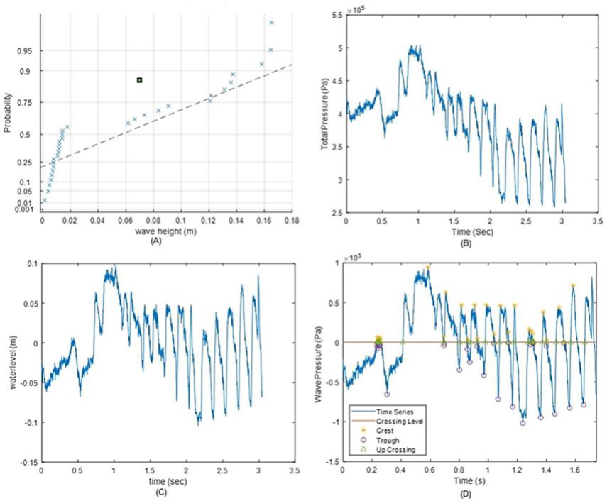
Figure 8 Wave record with a period of T=0.4771 Sec. A: The Rayleigh distribution of the pressure sensor, B: Total pressure caused by hydrostatic pressure and wave pressure, C: Wave surface profile
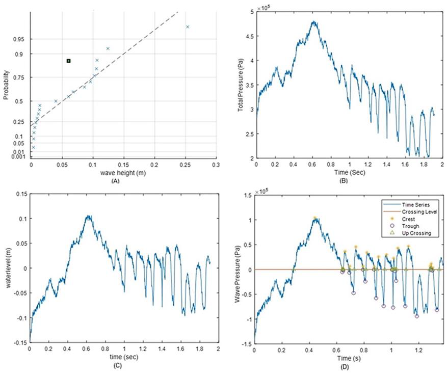
Figure 9 Wave record with a period of T=0.5576 Sec. A: The Rayleigh distribution of the pressure sensor, B: Total pressure caused by hydrostatic pressure and wave pressure, C: Wave surface profile

4.3. Based on PIV image (image processing)
4.3.1. PIV technique setup
The PIV setup is shown in Figure 11. A big sky double pulsed Nd: YAG (Neodymium-Doped Yttrium Aluminum Garnet) laser of wavelength 532 nm and 200 mJ/Pulse with the maximum repetition rate of 15 Hz per laser head was used to provide illumination of the seeding particles. The laser sheet adjustment is the most important step in PIV setup to obtain highly accurate results and safety issues. This was done using orange light-sensitive paper. That paper was placed in the front of the laser beam source in the middle of the flume tank (test section, the location where the laser sheet should be generated). The laser beam source was performed with a lower laser energy limit and was visible in the dark ambient light condition to ensure safety. The two laser beams sources should leave marks on the orange paper. One mark was found on the orange paper, which means two laser beams are hitting at the same point (LaVision GmbH, 2016). The laser beam source was directed from above the flume tank towards the middle of the water surface using a 45( dielectric mirror, then a cylindrical lens was used to convert the laser beam into the laser sheet with a thickness is about 2 mm.

The laser sheet was generated to be perpendicular to the water surface and parallel to the sidewall of the flume tank. The laser sheet was slightly inclined at a 6( downwind from the middle of the flume tank. LaVision charged coupled device (CCD)Imager Pro X 2m camera was used. The camera resolution is 1600 x 1200 pixels with a bit depth of 14 bit, and the pixel size is 7.4(m. The camera has a double exposure feature with an interframe time down to 100 ns, and the frame rate is 30 fps at full resolution. The camera is fitted with an adapter to connect it with a NIKON AF NIKKOR zoom lens (50 mm 1:1.8 D), which means the focal length is 50 mm, and the f- stop number is 1.8. Camera alignment is a critical issue that can affect the accuracy of the measurement. Thus, the CCD camera should be set with the optical axis perpendicular to the laser sheet. The misalignment between a CCD camera and the laser sheet produces a bias in the measurements (Kompenhans et al., 2002; Raffel et al., 1996; Scarano, 2013). The camera was mounted in the front of the flume tank with a 6( inclined angle from the perpendicular axis, as shown in Figure 12.

The calibration algorithm in Davis (8.4) was used to calibrate the CCD camera to make sure the camera was arranged perpendicular to the laser sheet. HGS-10 hollow glass sphere with diameter 10(m and the density of
This experiment was done at the fluid dynamic laboratory at WMU, and the laboratory was completely dark when the PIV images were taken to reduce the illumination variability. This was done by covering the backside of the Acrylic Plexiglass flume tank with black paper, covering all lab windows with black plastic sheets, and turning off the light inside the lab.
4.3.2. Analyzed images captures using the PIV technique
The wave images at three different frequencies were captured using PIV techniques, as was explained above. As was illustrated before, the main objective of this method is to obtain wave height and wavelength. Due to space limitations at the front of the wave in the test section, it was not able to increase the field of view and capture a full wavelength. Thus, Matlab code was built to create a full wavelength from many successive PIV images. The Canny edge detection algorithm technique with the constant threshold value was used to detect the edge of the wave (water surface elevation) (Kamanga, 2017; Lee et al., 1987; Marques, 2011; Marr & Hildreth, 1980; Shokhan, 2014). Also, by using Matlab, the minimum points (trough) and maximum point (crest) at the one full wavelength were determined. Then, the values of wavelength and wave height were obtained by using the definition of wavelength (distance between two successive troughs) and wave height (the distance between crest and trough). Finally, to ensure that accurate results were evaluated, the final value of wavelength and wave height was calculated by taking the average of ten values obtained from ten trials, as is shown in Figure 13.

5. Results and discussion
The current study investigates the performance of three different methods which could be employed to measure the characteristics (specifically wave height and wavelength) of the intermediate water gravity waves generated mechanically in the flume tank. The methods proposed include making use of the wavemaker transfer function, the wave-induced pressure, and PIV-based image processing to obtain the wave characteristics. Table 2 shows the value of the wavelength and wave height obtained from analyzing the PIV images as explained earlier in section 4.2.3.
Table 2 The wave characteristic calculated based on the PIV images analysis.
| Parameters, m | Period T= 0.4771 sec | Period T= 0.5576 sec | Period T= 0.9585 sec |
| Wavelength | 0.357989 | 0.474643 | 1.083282 |
| Wave height | 0.069296 | 0.059355 | 0.02672 |
Dispersion theory was used to evaluate wavelength then substituted back into wavemaker transfer function Equation 21 to get the value of wave height. Wavelength cannot be directly solved for a given set of wave period (T) or still water depth(h) from dispersion theory. Thus, to get the value of wavelength, it should be found by iteration. In this study, four numerical methods were used to get wavelength, and the percentage of error was calculated relative to the value of wavelength and wave height obtained by analyzing PIV images that were considered as the true value of the wave measurements. The four most common numerical methods found in the literature that are used to evaluate wavelength are Newton Raphson method, Hunt method, Eckart method, and Approximation method. As shown below in Table 3, the smallest deviation was given by using the Newton Raphson method, followed by the Hunt Method.
Table 3 The wave characteristic calculated based on the flap wavemaker theory.
| A: - Wave period (T)= 0.4771 sec, wavelength (L)=0.357989 m, Wave height(H)=0.069296 m | ||||
| Type of method | Wavelength was calculated using dispersion relation, m | Percent of Error % (L) | The wave height was calculated using transfer function of flap wavemaker, m | Percent of Error % (H) |
| Newton Raphson | 0.358 | 0.0272 | 0.07310 | 5.489 |
| Hunt | 0.357 | 0.1918 | 0.07316 | 5.576 |
| Eckart | 0.359 | 0.2207 | 0.0730 | 5.345 |
| Approximation | 0.355 | 0.9575 | 0.07343 | 5.966 |
| B: -Wave period (T)= 0.5576 sec, wavelength (L)=0.474643 m, Wave height(H)=0.059355 m | ||||
| Newton Raphson | 0.475 | 0.0264 | 0.06183 | 4.169 |
| Hunt | 0.474 | 0.1495 | 0.06191 | 4.3046 |
| Eckart | 0.480 | 1.0274 | 0.06139 | 3.4285 |
| Approximation | 0.468 | 1.3379 | 0.06244 | 5.198 |
| C: - Wave Period (T)= 0.9585 sec, Wavelength (L)=1.083282 m, Wave Height(H)= 0.02672 m | ||||
| Newton Raphson | 1.084 | 0.0342 | 0.02824 | 5.6886 |
| Hunt | 1.0836 | 0.0311 | 0.02824 | 5.6886 |
| Eckart | 1.140 | 5.2580 | 0.0267 | 0.07485 |
| Approximation | 1.093 | 0.8714 | 0.0279 | 4.2723 |
The experimental data recorded using Honeywell pressure sensor were analyzed using Matlab software. Two Matlab codes were built to avoid manual calculation and get an accurate value of wave height, as shown in Figures 8 through 10, and were evaluated at three different wave frequencies. Then, the wavelength was obtained by using a dispersion relationship that was solved by using the Newton Raphson numerical method. The results obtained from pressure measurements and comparing these results with the results evaluated based on analyzed PIV images are summarized in Table 4.
Table 4 The wave characteristic calculated based on pressure measurement.
| Type of method | Wavelength was calculated using dispersion relation, m | Percent of Error % (L) | The wave height was calculated using Pressure Measurement, m | Percent of Error % (H) |
| Newton Raphson | 0.354 | 1.2128 | 0.0699 | 0.8716 |
| B: -Wave Period (T)= 0.5576 sec, Wavelength (L)=0.474643 m, Wave Height(H)=0.059355 m | ||||
| Newton Raphson | 0.478 | 0.7984 | 0.06183 | 4.169 |
| C: - Wave Period (T)= 0.9585 sec, Wavelength (L)=1.083282 m, Wave Height(H)= 0.02672 | ||||
| Newton Raphson | 1.083 | 0.0041 | 0.0244 | 8.683 |
Noteworthy to notice that the Newton Raphson numerical method is the best equation that can be used to solve the dispersion relation with the smallest deviation compared to values obtained based on analyzing PIV images were considered as the true value of wavelength and wave height. The percentage of deviation of the values produced by using the Newton Raphson method obtained based on the pressure measurements were ranging between (0.0264-0.0342) percent for wavelength and (4.169-5.6886) percent for wave height. Whereas values obtained based on the wavemaker transfer function were ranging between (0.0244-1.2128) percent for wavelength and (0.8716-8.683) percent for the wave height.
6. Conclusion
Waves were generated mechanically by a flap-type bottom-hinged paddle mounted at one end of the wave flume tank, which travels down the trough and is expected to dissipate smoothly on the slope of the beach, or it can be called a wave absorber. This experiment employed three different methods to obtain the characteristic wave parameters like wave period, wavelength, and wave height: based on the theory of flap-wavemaker transfer function, pressure measurements that were evaluated from the Honeywell pressure sensor readings and based on PIV images that were analyzed using Matlab software and the concept of canny edge detections. This experiment was focused on getting the direct value of wavelength and wave height and eliminating the errors that may produce by solving dispersion relation theory by one of the numerical methods. Then, the comparison between these methods was made and the percentage of error was calculated to evaluate the performance of these methods to get accurate wave measurements. Pressure measurements-based methods are conventional methods, point measurements, intrusive, and sometimes it is very hard to set up. At the same time, the transfer function of the flap wavemaker is valid only when the frequency of the flap wavemaker is the same as the frequency of the regular waves generated inside the wave flume tank. The PIV technique can be applied easily in the area of interest, reduces spatial sampling cost, and is valid for regular and irregular waves. The accuracy of the results obtained by analyzing the PIV image is strongly affected by the quality of PIV images, the performance of edge detection algorithms used, and the PIV setup (seeding, CCD camera, and camera calibration) (Viriyakijja & Chinnarasri, 2015). It is noteworthy to observe that the accurate value of wavelength and wave height obtained based on the pressure measurements and wavemaker transfer function are strongly dependent on the numerical method that should be used to solve the dispersion theory. Noteworthy to notice the most accurate results can be evaluated by employing the Newton Raphson numerical method.

