


 nueva página del texto (beta)
 Inglés (pdf)
 Artículo en XML
 Referencias del artículo
 Enviar artículo por email
 Citado por SciELO
  Similares en
SciELO
Similares en
SciELO 
 Permalink
Introduction
Regarding the Cobb-Douglas production function, originally presented in 1928, the joint shares of capital and labor are represented by net income. Under this framework annual additions to fixed capital in manufacturing are measured in dollars, and labor is measured in average number of wage-earners employed in manufacturing. Hence, the Cobb-Douglas function is bifactorial. While these authors are regarded as pioneers attributing net income to the above mentioned determinants, Douglas acknowledge that Wicksteed developed beforehand the above mentioned functional form.1 In formal terms:
where
Cobb and Douglas (1928) use a logarithmic scale to show the relative growth in manufacturing of fixed capital on equations (5) and (6). Doing the same time on both sides of equation (1) gives:
The simulation algorithm implemented in this paper uses Restricted Ordinary Least Squares (ROLS), which are applied to the linear processes described on equation (2). As reported in the results section, simulation estimates are identical to the published by Cobb and Douglas in 1928.
The Cobb-Douglas production function attempts to measure the effect of changes in the amount of labor and capital stocks which have been used to produce a certain level of income, and to determine the relationships existing between them, as well as the net product as an outcome (Cobb and Douglas, 1928). These authors inform that:
“...if the relative supply from year to year of labor and capital were thus even approximately ascertained, a number of further problems would inevitably present themselves for solution: (1) Can we estimate, within limits, whether this increase in production was purely fortuitous, whether it was primarily caused by technique, and the degree, if any, to which it responded to changes in the quantity of labor and capital? (2) May it be possible to determine, again within limits, the relative influence upon production of labor as compared with capital. (3) As the proportions of labor to capital changed from year to year, may it possible to deduce the relative amount added to the total physical product by each unit of labor and capital and what is more important still by the final units of labor and capital in these respective years? Might at least an historical approach to the theories of decreasing imputed productivity (diminishing increment to total product) be afforded and the way opened for further attempts to secure quantitative approximations to these assumed tendencies, if indeed there should turn out to be historical validity to them? (4) Can we measure the probable slopes of the curves of incremental product which are imputed to labor and to capital and thus give greater definiteness to what is at present purely an hypothesis with no quantitative values attached? (5) Finally from such a study of (a) the imputed physical product from year to year of a unit of labor and capital when joined with (b) a study of the relative exchange value of a physical unit of manufactured goods in these years and compared with (c) the actual movement of ‘real’ wages in manufacturing and of real interest (if the latter can be ascertained), may we secure light upon the question as to whether or not the processes of distribution are modeled at all closely upon those of the production of values?”
Cobb and Douglas (1928) assume that equation (1) is homothetic of degree one, meaning that α + β = 1. Therefore, this assumption describes an economy with constant returns to scale.3 According to Kmenta (1967), constant returns to scale assumption makes possible to estimate the elasticity of substitution from the marginal productivity condition by regressing the value of production per worker on the wage rate, with both variables measured in logarithms.
If the two factors of production are accounted for, their income sum will be equal to the value added to the total physical product by each unit of labor and capital (Cobb and Douglas, 1928, p.140).4 Examples of this accounting exercise are the input-output matrices, which are calculated at the end of a given accounting year. Is worth mentioning that input-output matrices reach an ex-post equilibria as product, demand, and supply are found to be equal.5 These equilibria could be addressed through three accounting phases in the literature. The first one refers to the sphere of production; the second one deals with production from the perspective of demand, and the third one takes as a scope the supply side. In these three accounting phases the Cobb-Douglas production function is frequently used to measure either increases in production or economic growth. The Cobb-Douglas production function estimation helps to determine the production factors shares α, β and total factor productivity η.6 This estimation draws conclusions which could become hypothesis. For instance, Skevas (2022) mentions that farms factor productivity evaluation and its drivers constitute an essential exercise. Thus, a Cobb-Douglas evaluation could help poorly performing farms to identify the production factors that could enhance their total factor productivity. These accounting equilibria phases are described briefly in what follows.7
The demand-supply accounting phase is permeated by the Keynesian theoretical approach. From the demand side, expenditure is the most important factor in determining economic activity.8 From the supply side, income is a distributive determinant. Under this accounting phase the following equation is conceived:
where
The supply-product accounting phase also follows the Keynesian logic. In this case, the input-output matrix rows accounts for labor, capital, and government incomes.9 Here, the supply dynamics is decisive to shape the patterns of income distribution.
where
In recent decades, there has been a change in the macroeconomic representation of the original Cobb- Douglas production function described in equation (1). Many economists identify this macroeconomic representation with an IS-LM (Investment Savings-Liquidity Preference Money Supply) theoretical framework.10 Real Business Cycle models (RBC) represents the economic phenomena with microeconomic foundations.11 RBC models analyze individual agents’ economic activity -microeconomics, or alternatively their aggregation-macroeconomics. Under RBC models, equation (1) could be analyzed either at a macroeconomic or microeconomic levels.12
The objective of this paper is to attain an algorithm that simulates the original Cobb-Douglas estimations for the period of 1899-1922 using Restricted Ordinary Least Squares (ROLS). Later the algorithm and Cobb- Douglas (1928) estimators are compared to verify that they are identical. Afterwards, this algorithm is used to make a contemporary application to the United States and Mexico annual data. Hence, the results from this contemporary application are read in the same way as Cobb and Douglas did with their 1928 estimates.
Critics to the Cobb-Douglas production function
Not all the economic literature shares the view that a Cobb-Douglas production function is useful to measure and quantify the production relationships. One source of criticism is tied with the constant return to scale assumption, since it imposes a rigid functional form with a lacuna of empirical evidence. Hence, for Kmenta (1967), whether constant returns to scale are typical or not is largely an article of faith. Other source of criticism is point out by Qiu et al. (2023) who mention that technological progress is critical to the growth of total factor productivity,13 but that this hypothesis is inconsistent with reality since most countries experience a bias towards technological progress. Regarding the income distribution imbedded in the Cobb-Douglas production function, Berndt and Christensen (1973) criticize that its functional relationship structure relays in the separability, substitution, and aggregation assumptions of the production factors which are found under perfect competition, while empirical studies point out the absence of perfect competition assumptions in the real world.
Other sources of criticism to the Cobb-Douglas production function claim that it is just an accounting exercise. Felipe and Adams (2005) recount a list of criticisms made by Samuelson (1979) regarding the Cobb-Douglas production function empirical verification, like multicollinearity, outliers, absence of technical progress, and aggregation of physical capital. Also, there is the critique that the Cobb-Douglas production function describes an income identity only in macroeconomics terms, since aggregation faces heterogeneity in labor and capital. Felipe and McCombie (2020) and Phelps-Brown (1957) show that cross-sectional estimates of production functions are predetermined: the results are known ex-ante by an accounting identity that relates output, employment, and capital stock.
This document is organized as follows: Section 2 presents a theoretical foundation of the Cobb-Douglas production function, where its assumptions, the theoretical production factor shares in the product, and their complementarity are established for a constant returns to scale economy. Section 3 is devoted to data analysis with descriptive statistics and figures. Section 4 contains the methodology of the simulation algorithm. Section 5 reports the econometric results. In the last section the discussion and conclusion are put forward.
1. Theoretical foundations
Equation (1) represents the Cobb-Douglas production function in its most frequent format. In this equation, the public sector and the external sector are omitted.14 From the national accounts approach equation (1) or alternatively equation (2) represent the reduced forms of an economy, with the omitted sectors just mentioned.
In 1927, Charles Cobb (1875-1949), mathematician and economist, and Paul Douglas, economist, and U.S. senator (1892-1976) presented this formulation which bears their names at the 40th Annual Meeting of the American Economic Association. In March 1928 they published their article “A Theory of Production”. Ever since, the use of this production function has become popular in economic academia both at the macroeconomic and microeconomic levels. The Cobb-Douglas production function in these authors notation is as follows:
where P is an index of the physical volume of manufacturing, b is a constant corresponding to what is nowadays identified as technology, L is an index for the probable average number of wage-earners employed in manufacturing, C is an index of the estimated annual additions to fixed capital in manufacturing in constant terms, k is the labor share in the product, 1 - k is the capital share in the product. Taking logarithms on both sides of the equation:
Calculating the partial derivatives of the last expression, with respect to the logarithm of each of the production factors the following shares are found:15
It is worth mentioning that k and 1 - k are empirically represented by the estimates
According to Velupillai (1973) and Sandelin (1976) the original formulation of the Cobb-Douglas production function is found on Knut Wicksell (1851-1926), although this is not widespread. Wicksell presented a formulation of the production function in 1916 in the Economic Tidskrift, in his article Den "kritiska punkten" i lagen för jordbrukets aftagande produktivitet (The "critical point" of the law on diminishing agricultural returns). The production function presented by Wicksell (1916) is reproduced next:
where
It is worth mentioning that a difference between the production functions of Wicksell and Cobb-Douglas is the land production factor, although their exponential forms are the same. That is, equations (5) and (9) are identical if the land production factor is eliminated and if the same notation is used. The Wicksell production function was hardly widespread. Perhaps the reason is due to the language of dissemination of the original articles. Cobb-Douglas work was in English and Wicksell in Swedish.
In the theoretical formulation of the Cobb-Douglas production function, the quantities of the production factors labor and capital are exogenous, meaning that they are determined by the available technology and do not depend on the endogenous decisions made by the producer. In the other hand, when income distribution is analyzed, payments to the factors of production are endogenous to the production process. Considering perfect competition assumptions, capital share is represented by its marginal productivity 1- k in equation (7). This marginal productivity is represented in the market by the interest rate paid on capital flows, or in the national accounts by the Gross Operating Surplus net of capital depreciation. Under the same set of assumptions, labor share is represented by its marginal productivity
As mentioned before, the Cobb-Douglas production function assumes constant returns to scale. This theoretical framework does not explain capital dynamics within a given year. To explain product fluctuations and economic growth with this type of function, some authors introduce modifications to it using stochastic calculus to explain short-term production fluctuations. Despite these modifications, the amount added to the total physical product by each unit of labor and capital is inescapably determined in an accounting manner by the amounts of capital and labor used in the whole accounting year. RBC models deal in more detail with describing output fluctuations, which in their framework are caused by random exogenous shocks and not by short-term fluctuations in the capital stock. Here, random exogenous shocks are imputed to possible market failures.
It is assumed that the capital factor can be accounted for in each production period net of depreciation.16 The capital growth rate is then the gross fixed capital formation as a flow, net of depreciation.17 Capital valuation is more complex at market prices, involving interest rates, stock market value, book value, discounted flow of expected earnings from an investment either in physical or financial assets, original cost of using the capital factor in productive investments, or acquisition cost. If profits are a production cost in perfect competition, then they are determined by the marginal capital productivity 1- k, or its share in the product
It is assumed that labor receives a monetary rent for the labor force paid at some point in the production cycle. For example, the derived demand for labor does not precede production implying that labor is considered only for the period in which the production is carried out. From the point of view of income distribution theories in equation (4), wages are distributed once the production cycle has ended. From the perspective of production, i.e., equations (1) and (6), under perfect competition, wages are the marginal productivity of work accrued at the time of production. In the labor market, labor is accounted as identical to units of working hours, that is, in physical units which in turn can represent quantities of product that workers demand, i.e., equation (3). This view has been explored by Ohlin (1967) who mentions that “The price of the goods a worker buys is the cost of his labor to the employer”.18 It is important to mention that in this frame labor is believed to be a service. However, in the primary and secondary sectors of the economy, the result of labor is a value added embodied in a physical form of a good that did not exist before. Therefore, as a product it has a specific physical form, suitable for storage. Therefore, labor can be considered from different analytical perspectives.
Given the series of previous assumptions in which the Cobb-Douglas production function and the factors of production construct, it is found that in equations (1), (2), and (3), the product is exhausted: either on consumption of the product (accounting phase one), or in factor income distribution (accounting phase two). In addition to these assumptions the law of markets is imposed on the product and each one of the factors of production, since the Cobb-Douglas production function is always represented as an equality. If one market is in equilibrium, then instantly the rest of markets will be also in equilibrium by Walras law. If all markets clear, then they are efficient, and the general economic equilibrium is achieved. Here, the corollary would appear to be the premise.
Continuing with the notation used in equation (1), the profit function can be written as follows:
where
In the long run, perfect competition considers that profits are equal to zero
Equation (11) is known as one version of the Euler's theorem. If the equality expressed in equation (12) is maintained, it can be inferred that all the product is exhausted in the payment to the production factors. Equations (11) and (12) are equivalent since they are equal on the right-hand.
From equation (2) the shares of each production factor can be calculated as has already been shown in equations (7) and (8). These equations are rewritten using the notation of equation (2).
Cobb and Douglas (1928) deduce that the productivities of each factor of production are equal to the shares of labor and capital on the product. Also, they demonstrate that these shares are constant proportions of the product. Considering equations (1) and (12) they are equal to Y on their left-hand sides, assuming a normalized product price p = 1. Therefore, the shares of labor and capital in the product can be expressed as follows:
If equation (11) holds, total production costs are equal to the expenses on the factors of production, where the right hand side of equation (11) is the sum of the left hand side of equations (15) and (16). Furthermore, consider that equations (10) and (11) are equivalent as explained above. Then, if equations (15) and (16) are substituted into equation (10), the following equation can be obtained:
If p = 1, then equation (17) can be rewritten as follows:
Equation (18) expresses an equality between the productivities of total labor
Considering equations (15), (16), (19), and (20) the shares of labor and capital in the product are equal to the partial derivatives of the Cobb-Douglas production function, as expressed below:
The shares of the production factors are equivalent in the three different accounting phases reviewed: the first accounting phase dedicated to the production sphere, i.e., equation (18). Also, they can be considered in the accounting sphere of demand (expenses), or costs, illustrated by equation (11). Finally, the supply sphere or income distribution, as shown in equation (12).
The Cobb-Douglas production function expressed in equation (1) is an idealized expression of a production process. In this case, equation (1) is, as mentioned before, a bifactorial function on capital and labor. The labor share in the product necessarily entails a complementary participation with the capital share, if a homogeneous Cobb-Douglas production function of degree one is assumed. This complementarity is clearly expressed in equation (12) since the product is exhausted in the production factors payment. Thus, the sum of the production factors shares must give one, based on what has been assumed. Thus, dividing both sides of equation (18) by
Equation (23) expresses that the production factors share in the product is always constant, since their sum is equal to one expressing then constant returns to scale. Equation (23) shows how the participation of the production factors is complementary since their sum is equal to one, and at the same time provides an expression where the factor shares can be read as percentages:
III. Data
This section describes the main trends in total shares of capital and labor factors on the product. Descriptive statistics are provided for three empirical cases. The first empirical case refers to the original Cobb-Douglas data for the United States economy during the period from 1899 to 1922. The second and third empirical cases refer to the United States and Mexican economies for the periods of 1993-2019 and 1993-2015, respectively. All data bears an annual frequency. Tables 1, 2 and 3 show descriptive statistics for each case.
Table 1 United States. Participations of capital and labor in the product. Annual frequency: 1899-1922 (1899=100)
| L/Y | K/Y | |
|---|---|---|
| Mean | 77.00 | 13.00 |
| Maximum | 100.00 | 49.00 |
| Minimum | 43.00 | 4.00 |
| Coefficient of variation | 0.21 | 0.86 |
Source: own elaboration based on Cobb and Douglas (1928).
Table 2 United States. Participations of capital and labor in the product. Annual frequency: 1993-2019 (1993=100)
| K/Y | L/Y | |
|---|---|---|
| Mean | 1.07 | 0.21 |
| Maximum | 1.13 | 0.38 |
| Minimum | 1.00 | 0.00 |
| Coefficient of variation | 0.03 | 0.66 |
| Y is an index of the Gross Domestic Product (GDP), L is an index for the aggregate weekly hours of employees in production, and K is an index of the net stock of fixed capital and consumer durables. | ||
Source: own elaboration based on the Bureau of Economic Analysis, and the Bureau of Labor Statistics.
Table 3 Mexico. Participations of capital and labor in the product. Annual frequency: 1993-2015 (1993=100)
| K/Y | L/Y | |
|---|---|---|
| Mean | 1.01 | 0.11 |
| Maximum | 1.04 | 0.23 |
| Minimum | 0.94 | 0.00 |
| Coefficient of variation | 0.03 | 0.62 |
| Y is an index of gross value added in basic values, L is aggregate working hours of employees, K is the net stock of capital. | ||
Source: own elaboration based on INEGI.
In Table 1 the largest mean is hold by the labor participation with an average of 77 for the period 1899 to 1922. Meanwhile, the lowest mean is for capital participation with a value of 13 for the same period. Regarding the coefficient of variation, labor participation reports a value of 0.21, which is much lower than the corresponding for capital 0.86. These coefficients of variation indicate that capital participation has a greater dispersion around the mean in comparison to capital.
For the United States Table 2 reports the same descriptive statistics as Table 1, during 1993 to 2019. The data query is made in January 2023. Although there is data for labor until 2021, capital series are available up to 2019. Thus, capital data availability determines the cut-off year for the data reported. The starting year for this period is 1993, to maintain parsimony with Mexican available data.
In Table 2 the largest mean belongs to capital participation with a value of 1.07, for the period from 1993 to 2019. Meanwhile, labor has the lowest mean with a value of 0.21 for the same period. Regarding the coefficient of variation, capital participation has a value of 0.03 which is much lower, than the corresponding labor coefficient of variation of 0.66. These values indicate that labor participation has a greater dispersion around the average, than the capital factor. Probably, the labor market is more unstable than the capital market.
Table 3 refers to similar descriptive statistics as in Tables 1 and 2. Now, Mexico is the economy under analysis for the period from 1993 to 2015 with annual observations. Data retrieval was performed on January 2023: capital data is available up to 2021, while labor and output are only available up to 2015. For this reason, 2015 is the cut-off year for the Mexican data reported in Table 3.
Table 3 shows that the largest mean is for the capital participation of 1.01, considering the period from 1993 to 2015. Meanwhile, the lowest mean is for labor with a value of 0.11. Regarding the coefficient of variation, capital reports a value of 0.03, which is much lower than the corresponding coefficient of variation of the labor participation of 0.62. Thus, probably the labor market is more instable than the capital market.
Next, five figures depict the times series evolution for the total participation of the factors of production capital and labor in the product, whose descriptive statistics are reported on Tables 1-3. Figure 4 makes a comparison between the total participation of the labor production factor in the product for the United States and Mexico. Figure 5 makes a comparison between the total participation of the capital factor in the product for these economies.
In Figure 1 the total participation of labor increases over time from values close to zero to fifty, towards the end of the period. The first years is the baseline for these indexes. The main trend of capital participation is decreasing during the period under analysis, going from one to 0.20 in 1921.
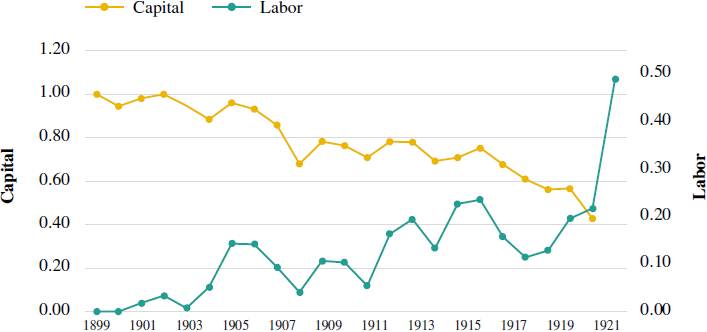
Source: own elaboration based on Cobb and Douglas (1928).
Figure 1 United States. Participation of capital and labor in the product. Annual frequency: 1899-1922 (1899=100)
In Figure 2, the trend of labor participation in the product is increasing, going from values from zero to forty percent. Figures 1 and 2 show that the total participation of labor decreased by about ten percent at the end of each period. Income distribution worsened for labor participation in this last period. For its part, capital participation is growing during the period analyzed, going from one in 1993 to about 1.12 in 2019, falling perhaps due to the rise in world oil prices in 2001 (Campodónico, 2001), and the Great Recession in 2009. Figures 1 and 2 show that factor participation trends reverse from Figure 1 to 2, meaning that during the last period the income distribution for capital has improved, while labor participation has worsened.
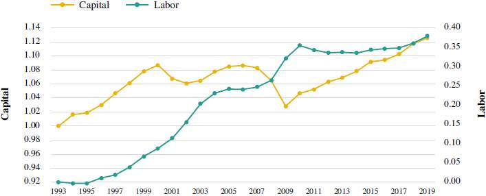
Source: own elaboration based on Bureau of Economic Analysis and Bureau of Labor Statistics.
Figure 2 United States. Participation of capital and labor in the product. Annual frequency: 1993-2019 (1993=100)
Figure 3 presents the capital and labor participation in the product for Mexico. Labor participation increases during the period of 1993-2015, since it goes from values close to zero percent to around 25 percent. Regarding the capital participation, it has ups and downs in its behavior with substantial short-term falls in 1994, 2001, and 2009 which are linked to the devaluation of the Mexican peso, because of the Tequila Effect, the rise in the oil price, and the Great Recession, respectively. The minimum value of it is 0.94, while its maximum value is 1.04, indicating that its dispersion around the mean (1.01) is not larger.
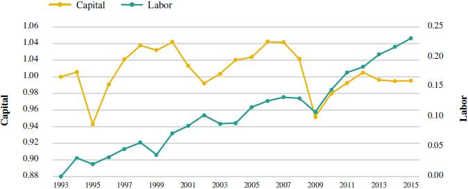
Source: own elaboration based on INEGI.
Figure 3 Mexico. Participation of capital and labor in the product. Annual frequency: 1993-2015 (1993=100)
Figure 4 shows that labor participation in the United States is largest with 35 percent in 2015, than in Mexico during the period under analysis having 1993 as base year. Meanwhile, the same participation in the product for the case of Mexico grows modestly reaching values close to 25 percent.
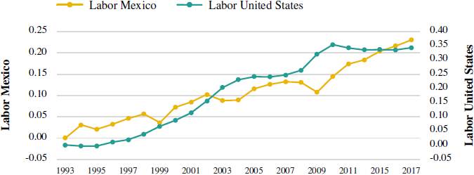
Source: own elaboration based on Bureau of Economic Analysis, Bureau of Labor Statistics, and INEGI.
Figure 4 United States and Mexico. Participation of labor in the product. Annual frequency: 1993-2015 (1993=100)
Figure 5 shows that capital participation in the product for Mexico and the United States are somehow similar. In 1994 capital participation fell in Mexico (from 1.03 to 0.945), while in the United States this share increased slightly (from 1.020 to 1.025). Global financial phenomena such as the rise in oil prices in 2001, and the Great Recession in 2009 affected in a similar fashion capital participation for both economies. The economy of the United States shows greater resilience to these types of external shocks, since it depicted the smaller coefficient of variation -Tables 2 and 3, in comparison to the Mexican economy.
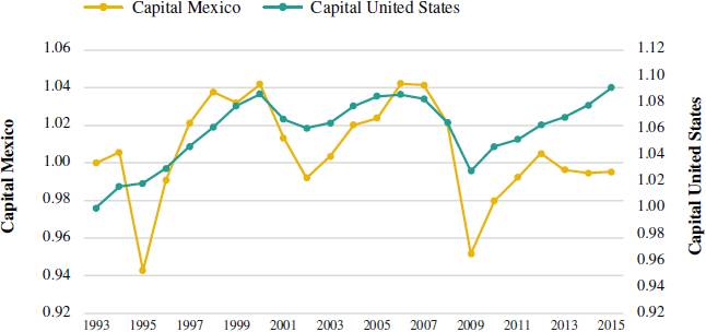
Source: own elaboration based on Bureau of Economic Analysis, Bureau of Labor Statistics, and INEGI.
Figure 5 United States and Mexico. Participation of capital in the product. Annual frequency: 1993-2015 (1993=100)
III. Methodology
Cobb and Douglas (1928) use least squares to estimate factor shares in the amount added to the physical product.19 The objective of this paper is to attain an algorithm that simulates the above mentioned factor shares for the period of 1899-1922 using Restricted Ordinary Least Squares (ROLS) since the condition of constant returns to scale is considered as a constraint. To do this, the annual time series corresponding to product, capital and work published by the previously mentioned authors are taken. Once the ROLS-based algorithm that reproduces the results of the same authors has been obtained, it will be used to make a contemporaneous application to the United States (1993-2019) and Mexico (1993-2015) cases. The analysis is carried out in the three above mentioned periods with an annual frequency. The previous procedure helps to interpret the results of these contemporary cases, in the same way as Cobb and Douglas did in 1928 with their data. Returning to equation (2), it is modified to introduce the subindex
where Y is the product, A is the technology,
By applying the logarithm function to all time series under consideration, it is possible to change the scale of the time series to logarithmic. Therefore, although different units are included in equation (25) such hours worked for labor, and millions of monetary units (US dollar and Mexican peso) for capital, the estimates obtained with this transformation are coefficients of elasticity.
Cobb and Douglas (1928) use a constraint concerning the marginal shares of the factors of production labor and capital in the product adding up to one, since they considered a production function homogeneous of degree one: “... Production is a first degree homogeneous function of Labor and Capital.” This constraint is expressed in equation (23), Cobb and Douglas (1928, p. 151), and in percentage terms in equation (24). This constraint is part of the ROLS estimation.
The hypothesis for the econometric model expressed in equation (23) is that the economies under analysis exhibit constant returns to scale. Then, if the hypothesis is true, η, which represents the estimator of total factor productivity must be equal to one. Being the case, it is verified that the corresponding economy exhibits constant returns to scale. If η is greater than one, it implies that there are factors of production whose accounting exceeds the reported product. If η is less than one, then there are factors of production whose accounting is omitted from the reported product.
According to the Bureau of Economic Analysis (BEA), gross value added (GVA) is made up of the sum of compensation to employees, gross operating surplus and net taxes on products and imports. From the previous definition, the sum of the shares of the factors of the Cobb-Douglas production function do not make up the total value added. If the constraint α + β = 1 is imposed, this means that the sum of the corresponding estimators will be one, but not that their sum is equal to the gross value added, as expressed in equation (17), since it represents only the sum of the shares of labor and capital factors on production, without net taxes on products and imports.
III. Results
The results of estimating the econometric model on equation (25) with ROLS are reported on Table 4. The first column of Table 4 is referred to the United States for the 1899-1922 period, while the second column is referred to the same country for 1993-2019. The third column exposes the result for Mexico during the 1993-2015 period.
Table 4 United States and Mexico. Regression results when applying the Restricted Ordinary Least Squares, equation (25). Annual data (Student's t statistic)
| Estimates | United States dependent | Mexico dependent | |
|---|---|---|---|
| logY 1 | logY 2 | logY 3 | |
|
|
101% (1.73)* |
104% (6.04) *** |
102% (2.53) *** |
|
|
25% (6.16)*** |
89% (21.93)*** |
82% (10.35)*** |
|
|
75% (18.09)*** |
11% (2.33)*** |
18% (2.30)*** |
|
|
0.057 | 0.0267 | 0.0243 |
| F | 1.69 (0.09)* |
1.09 (0.09)* |
2.95 (0.07)* |
| n | 24 | 27 | 23 |
| Period | 1899-1922 | 1993-2019 | 1993-2015 |
| RMSE stands for the Root Mean Square Error. Significance: ( )*** 99%, ( )** 95%, ( )* 90%. The F reported is the Breusch-Pagan/Cook-Weisberg test for heteroskedasticity with H 0: constant variance: in the three equations reported the presence of heteroskedasticity is rejected at the significance level of 95%. The Stata 18 program was used. The estimates are given in percentage terms. | |||
Source: own elaboration.
As shown in equations (1) and (2) the independent variables are technology, capital and labor. The estimates associated with each of these independent variables are η, α, and β, respectively. They are basically significant at 99%.
Regarding column one of Table 4, the estimates obtained after applying the algorithm to the data published by Cobb and Douglas (1928) are reported. This algorithm is found to provide identical results to those reported by these authors on page 151 of their paper:20
In what follows, equation (1) is rewritten, with the results reported in the first column of Table 4, without percentages and with rational expressions, obtaining:
From the previous two equations it can be verified that the algorithm implemented in Stata 18 reproduces the procedure applied by Cobb and Douglas in 1928. Then, this algorithm is applied contemporary to the cases of the United States regarding the 1993-2019 period, and for Mexico during the period 1993-2015. Using equation (1) again, the results reported in columns two and three of Table 4 are rewritten as:
Second column:
Third column:
Total factor productivity for the United States indicates an increased by about 3%,21 with respect to the two periods under consideration. For its part, Mexico presents a total factor productivity of 2%. In other words, Mexican productivity is below its United States counterpart, at least in recent times. In the case of China, Qiu et al. (2023) report that total factor productivity for the period of 1980-2000 is equal to 0.965, i.e., close to one.
The importance of these estimates for policy making is underlined by Felipe and Adams (2005).22 Fagerberg (2000) demonstrates that countries that have managed to increase their presence in the technologically most progressive industry in this period -electronics- have experienced higher productivity growth than other countries, on the order of 0.03 to 0.07. He mentions that the relevant policy conclusion to draw from this is not that every country should move into production of electronics as fast as possible, without considering the existing national assets and capabilities. Mallick (2012) results suggest that both theoretical and empirical research on economic growth should pay more attention to the role of the constant elasticity of substitution parameter and reconsider the usefulness of the Cobb-Douglas production function in growth theory. For its part, Xu et al. (2020) perform empirical research reported in their Table 2, demonstrating that total factor productivity is mainly attributed to technological progress driven by labor force. These authors design a policy allocation using delaying tax payment and proper tax policy allocation, thereof economic and social benefits of enterprises can be balanced, and total factor productivity can be promoted.
According to the hypotheses of the econometric model, economies with constant returns to scale should be observed by imposing the restriction that the shares of the factors of production are equal to one when implementing ROLS. However, the total factor productivity reported in Table 4 exceeds one by 1%, 4%, and 2%, in each column respectively. Perhaps, there are production factors that are omitted or poorly accounted among the independent variables. That is, the product is greater than the sum of the factors of production shares labor and capital. This result is not new. Solow (1957) points out that total factor productivity represents a residual, since its existence is not linked to the accounting of capital and labor factors. According to Solow (1957), the residual represents an approximation to technological change, which could be caused by unaccounted production factors, such as technological innovation and environment interactions.23 Rearranging equation (23):
where η = 1. Applying equation (30) to each column of Table 4 yields: First column:
Second column:
Third column:
If the residual is understood as a technological innovation, then total factor productivity has grown in the United States from one period to the next by 3%. Meanwhile, for the last period available in both countries technological innovation has been lower in Mexico (2%), in comparison to the United States (4%). Francis et al. (2020), using a Cobb-Douglas specification applied to the Enterprise Survey World Bank database claim that median size firms operate close to constant returns to scale, and that using either gross-output and value-added production functions provide similar ranking of sectors in terms of output elasticities, capital intensity and returns to scale.
Regarding the estimators of the production factors of capital and labor in the United States reported in Table 4, they revert their behavior from the period 1899-1922 to the period 1993-2019. That is, the income distribution change, if the Euler's theorem described in equation (12) applies alongside with all the Cobb- Douglas production function assumptions depicted in section II. For the United States in the first period labor share was 75%, while in the recent period it stands at 11%. In other words, the distribution of income for labor has worsened in recent times. Meanwhile, the capital share improves for the United States since it goes from 25% to 89%, for the two periods under consideration. These results are in line with Piketty (2014, 2021) who points out that there has been an income distribution in favor of capital in recent decades, not only in the United States but throughout the world. For example, in the case of Mexico for the 1993-2015 period, Table 4 shows that the capital factor is the one that takes the largest share in the product with 82%, while the share of the labor factor is 18%.
III. Discussion and conclusion
In the literature there are different measurements of the Cobb-Douglas production function or modifications of them, i.e., Felipe and McCombie (2012) make a list. This research takes the important step of using the original paper where the Cobb-Douglas (1928) production function is empirically measured. Thereby, this research omits variations in measurement outside the original Cobb-Douglas production function that have been appearing through time. The purpose of using the original Cobb-Douglas production function is to find an algorithm replicating the procedure initially followed by these authors. Once the algorithm that simulates the results published by Cobb and Douglas (1928) is verified, a contemporary application has been made for the United States and Mexico.
Descriptive statistics expose the evolution in the participation of the production factors with a base year. Here, the labor market is more unstable vs. the capital market. In recent times, capital has the largest participation in the product. The United States attains 1.07, while Mexico reached (1.01) in relation with the labor factor (0.21) and (0.11), respectively. A graphic analysis shows that income distribution worsened for labor in the United States during the two periods under analysis, the contrary has happened for capital. Global financial phenomena such as the rise in oil prices in 2001, and the Great Recession of 2009 have affected capital shares in both economies, while the economy of the United States shows greater resilience to these types of external shocks, than the Mexican economy.
Econometric estimates expose the production factors share evolution with a logarithmic scale. The capital and labor shares for the United States reported in Table 4 show an income distribution change. They revert their behavior from the period 1899-1922 in comparison with the period 1993-2019. In the first period, labor share was 75%, while in the recent period it stands at 11%. Therefore, its income share has been reduced in recent times. Meanwhile, capital share improves for the United States since it goes from 25% to 89%, during the periods under consideration. These results are in line with Piketty (2014, 2021) who points out that there has been a distribution of income in favor of capital in recent decades, not only in the United States but throughout the world. For example, in the case of Mexico for the period 1993-2015, Table 4 shows that the marginal participation of capital has the largest share in the product (82%), while labor share is 18%, similarly for the United States these figures are 89% and 11%. If the residual is understood as a technological innovation, then total factor productivity has grown in the United States from one period to the next by 3%. Contemporary data exposes that technological innovation has been lower in Mexico (2%), compared to the United States (4%). The behavior of factor shares by themselves continue to be a foremost element in terms of income distribution, considering the pattern evinced in recent periods.

