Pines have traditionally been identified and classified using morphological and anatomical characters from ovulated cones and leaves (Mergen et al. 1965, Hicks 1973, Abbott 1974, Xing et al. 2014). Additionally, morphometric studies have been used to identify species limits in taxa with a wide geographic range and high morphological variation (Stead 1983, Matos 1995, Callaham 2013, Xing et al. 2014). Some studies have been successful (Abbott 1974, Xing et al. 2014), but some others have struggled with high variation among individuals and phenotypic plasticity (Pooler et al. 2002, Tauer et al. 2012).
There is ample literature on the phenotypic variation patterns along environmental gradients such as temperature and precipitation (Savolainen et al. 2007, Aparicio-Rentería et al. 2020, Leal-Sáenz et al. 2020). However, morphological characters not always respond to geographical or environmental variables in a linear manner (Malusa 1992, Cruz-Nicolás et al. 2020), but are the product of the interaction of local adaptation to microenvironments, gene flow, genetic drift, and population history (Borazan & Babaç 2003, Cruz-Nicolás et al. 2020, Uribe-Salas et al. 2008, Zúñiga et al. 2009). In such scenarios, species respond to those environmental challenges by maintaining high levels of genetic diversity and/or through phenotypic plasticity, in particular when individuals are long lived (Cavender-Bares & Ramírez-Valiente 2017).
Conifers tend to lack marked morphological differences in part due to incomplete reproductive barriers that allow for interspecific gene flow (Rehfeldt 1999, Carney et al. 2000, Gompert et al. 2012, Aguirre-Gutiérrez et al. 2015). Natural selection can either maintain the introgressed genes or force barriers to gene flow (Gompert et al. 2012), together with extrinsic factors depending on the fitness (Barton & Hewitt 1985, Hamilton & Aiken 2013, Janes & Hamilton 2017). Therefore, conifer species complexes represent a valuable system to test integrative taxonomy methods in order to delimit species and understand how diversity in populations is maintained.
Pinus ayacahuite Ehrenb. ex Schltdl. and Pinus strobiformis Engelm. are two species from the subgenus Strobus (Eckenwalder 2009), section Quinquefolia, subsection Strobus (Syring et al. 2007) which constitutes a species complex with similar morphological characteristics which has resulted in multiple synonyms and difficult identification (Kral 1993, Farjon & Styles 1997, Farjon 1998, Maya 2006, Eckenwalder 2009). Among the diagnostic characters that have been used for identification are the seed size, length of the seed wing, needle length, distribution, number of stomata, and seed cone morphology (Pérez de la Rosa 1993, Farjon & Styles 1997, Frankis 2009). Pérez de la Rosa (1993) examined 17 characters of the P. strobiformis-P. ayacahuite complex and found a pattern of clinal variation in the needle and seed wing length from North (P. strobiformis) to South (P. ayacahuite), with intermediate forms found in the Trans Mexican Volcanic Belt (TMVB). This result is supported by nuclear genetic markers that find evidence of introgression mostly in the populations of the TMVB (Moreno-Letelier et al. 2013, Moreno-Letelier & Barraclough 2015). This area is where Pinus veitchii Roezl has been described in temperate and humid mixed conifer forests between 2,600-3,100. Unlike the other two taxa, it has an extremely restricted distribution with fragmented stands in the states of Michoacán, Tlaxcala, Estado de México, and Morelos. P. veitchii was described from a population near San Rafael Tlalmanalco, on the slopes of the Iztaccíhuatl volcano, and it is also common also around the Popocatepetl volcano. Perry (1991) also described populations in Tlaxcala, Michoacán and around Mexico City. Farjon & Styles (1997) consider the same three populations, adding one in the Cerro El Zamorano in Guanajuato and another near the Zempoala lake in the state of Morelos, but lists the Michoacán population as P. strobiformis. The later shows that depending on the author, the populations of white pines from the TMVB can be assigned to either P. veitchii, P. ayacahuite, and even P. strobiformis, generating confusion among people doing conservation, reforestation efforts, and even Christmas tree production. The impact of not knowing the true circumscription of P. veitchii also makes it difficult to ascertain the true distribution of the species, which has caused that previous potential distribution models to either ignore the taxon all together (Laughlin et al. 2011, Moreno-Letelier et al. 2013, Shirk et al. 2018) or possibly overestimate its distribution (Aguirre-Gutiérrez et al. 2015). It is important to clarify the circumscription of P. veitchii, distribution and genetic relationships with the other Mexican white pines in order to adequately evaluate its conservation status and preserve local adaptations (Boluda et al. 2021).
Integrative taxonomy. Accurate identification and species delimitation of pine species is important for systematics, forestry, and conservation. A lot of work has been done at incorporating different sources of information to recognize species (Dayrat 2005, Padial et al. 2010). These approaches rely on a unified species concept: independently evolving lineages of metapopulations (De Queiroz 2007), which considers all sources of evidence as contributing to the identification of those lineages, without a priori considerations of what kind of evidence should prevail. In this context, it is important to re-evaluate how well morphological, genetic and environmental characters can differentiate the three taxa.
The high morphological variation and taxonomic controversies of the P. strobiformis-P. veitchii-P. ayacahuite species complex makes these taxa a good model to test how morphological and ecological characters help distinguish different lineages, particularly the ambiguous taxonomic position of P. veitchii in the TMVB. Our hypothesis is that P. veitchii is in a contact zone between P. strobiformis and P. ayacahuite, and therefore will have intermediate values in morphological, environmental, and genetic variables suggesting a hybrid origin. Our aim is to analyze the species complex using an integrative approach with morphological, ecological and genetic sources of information, based on the unified species complex.
Materials and methods
Plant Material. The plant material was obtained from field samples deposited in the Herbario Nacional MEXU, Instituto de Biología, UNAM (IB-MEXU) and are listed in Table S1. The specimens were evaluated as follows: 62 specimens from the main distribution area of P. strobiformis, 11 specimens from P. ayacahuite, and 23 specimens previously identified as P. veitchii by at least one author from the TMVB, plus one locality of P. strobiformis also named Pinus stylesii Frankis ex. Businsky (Table 1, Businský 2008).
Table 1 Populations from the Trans-Mexican Volcanic Belt and adjacent locations with uncertain taxonomic identity.
| Site | Perry 1991 | Pérez de la Rosa 1993 | Farjon & Styles 1997 | Farjon 2010 | Businský 2008 | Frankis 2009 | Bisbee 2014 |
|---|---|---|---|---|---|---|---|
| La Palma, Mich. | Pinus ayacahuite var. veitchii | Pinus ayacahuite var. veitchii | Pinus ayacahuite | ||||
| San Rafael, Edo. Mex. | Pinus ayacahuite var. veitchii | Pinus ayacahuite var. veitchii | |||||
| Texcaltitlán, Edo. Mex. | Pinus strobiformis var. veitchii | ||||||
| Popocatepetl, San Nicolás de los Ranchos, Edo. Mex. | Pinus ayacahuite | Pinus ayacahuite var. veitchii | |||||
| Calcahualco, N of Vaqueria, Ver. | Pinus ayacahuite var. veitchii | Pinus ayacahuite | |||||
| Cerro Zamorano, Guanajuato | Pinus strobiformis | Pinus ayacahuite var. veitchii | |||||
| Talpa y Cuale, Jalisco | Pinus ayacahuite var. veitchii | Pinus strobiformis | Pinus strobiformis | Pinus strobiformis | |||
| Cerro del Potosí, NL. | Pinus strobiformis | Pinus stylesii | Pinus stylesii | Pinus stylesii |
Morphological differentiation among P. strobiformis-P. veitchii-P. ayacahuite species complex. We used nine morphological and one dendometric characters which have been used to discriminate species in the genus Pinus: Peduncle Width (Wped), Apophysis Length (Lap), Umbo Witdth (Wum), Seed Length (Ls), Seed Wing Length (Lw), Seed Wing Width (Ww), Needle Length (Lleav), Needle Sheath Width (Wsh), Number of stomatal lines (Ladx) and Tree Height (Treehg; Pérez de la Rosa 1993, Delgado et al. 2007). The last character was obtained from information in herbarium collections and field observations.
Leaf measurements were taken from 15 needles taken at random from each individual (n = 99, Table S1). The needles were fixed in FAA (formaldehyde alcohol, 70 % ethyl alcohol) for observed the stomata lines and counted using a Nikon microscope to 60x in the IB-MEXU (the consulted vouchers are listed in Supplementary Table S1). Between 2-5 ovulated cones per locality of the three taxa were measured, with 10 scales and seeds from the central part of the cones. A total of 120 cones were measured.
Statistical analyses.- We obtained a Pearson correlation matrix of 9 morphological variables using the function “cor” with the corrplot package for R (Kendall 1938, R Core Team 2021, Wei & Simko 2021) and eliminated one of the variables of pairs with a correlation value > 0.8. After that filter, 9 variables were retained (Figure S1). The 9 variables retained, and the tree height were normalized by standardizing the arithmetic mean values with their z-scores of each one. This was done to ensure that each variable had an equal contribution in the different statistical and multivariate analyses. We used the functions included in the FactoMineR and factoextra packages (Lê et al. 2008, Kassambara & Mundt 2017).
We carried out a one-way ANOVA (Analysis of variance) and MANCOVA (Multivariate analysis of covariance) to establish if there are significant differences among the groups: P. strobiformis, P. veitchii and P. ayacahuite, as suggested by Delgado et al. (2007). The variables that were significant in a MANOVA (multivariate analysis of variance) analysis were retained for further analyses among groups.
A principal component analysis (PCA) was performed to analyze the morphospace of all individuals and to simplify the variance contribution of all variables. We used the FactoMineR and factoextra packages for R (Lê et al. 2008, Kassambara & Mundt 2017). All multivariate analyses were performed using R v. 3.4 (R Core Team 2021). The results were visualized using a UPGMA dendrogram (Sokal & Michener 1958) using PC1 and PC2 scores (Gailing et al. 2012).
A Linear Discriminant Analysis (LDA) was performed to select the morphological variables that had a greater contribution to the variance, using the highest PCA eigenvalues (>1) as a guide (Cabrera-Toledo et al. 2020). The LDA was used to assign individuals to any of the three groups (P. strobiformis, P. veitchii and P. ayacahuite). The classification success was estimated with a leave-one out cross validation (Nuzzo et al. 2022). The results are presented in a confusion matrix with the observed and predicted classifications (Cabrera-Toledo et al. 2020, Nuzzo et al. 2022).
Ecological divergence of the P. strobiformis-P. veitchii-P. ayacahuite species complex. The presence points of the P. strobiformis-P. veitchii- P. ayacahuite species complex were compiled from herbaria (IB-MEXU, CIIDIR-DURANGO, FCME of UNAM and UAMIZ-UAM), our own collections and the Global Biodiversity Information Facility (GBIF 2024). The following filters were applied to ensure reliable geographical information (Martínez-Méndez et al. 2016): 1) elimination of duplicate records and those with incomplete information, 2) elimination of inaccurate coordinates or those with atypical geographic locations (outside distribution range, cities, water bodies), 3) all records closer than 5 km were eliminated to avoid spatial autocorrelation using the Wallace package (Kass et al. 2018). The total number of records used for further analyses were: P. strobiformis (135 records), P. veitchii (13 records), and P. ayacahuite (85 records, Figure 1).
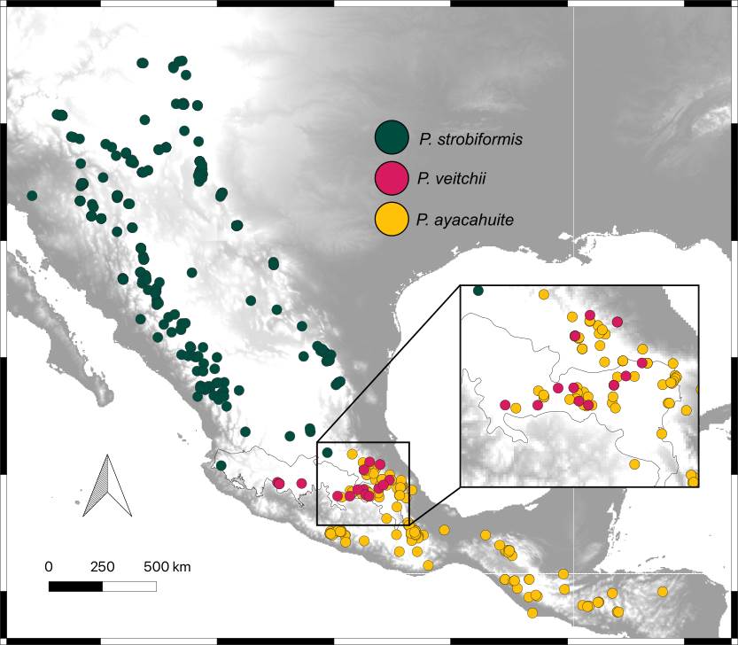
Figure 1 Distribution of the Pinus strobiformis-Pinus ayacahuite species complex. Dots represent the distribution of specimens (IB-MEXU and FCME of UNAM, and CIIDIR-Durango), field collections and GBIF data.
The environmental variables used were the 19 bioclimatic variables from WorldClim (Fick & Hijmans 2017) The resolution of all layers was 2.5 min. We used the Variation Inflation Factor (VIF, Brauner & Shacham 1998) to determine how variance is increased in a regression due to multicollinearity. Variables with values over 10 were discarded (James et al. 2014, Bruce & Bruce 2017). A one-way ANOVA and a Principal Component Analysis were performed on the retained variables to identify significant differences among species. All analyses were performed with the package FactoExtra and FactoMineR for R v. 3.4 (R Core Team 2021).
Based on the VIF multicolinearity analysis, the variables that were kept (Values <10) for the ENMs were: Average diurnal temperature range (Bio1), Mean Diurnal Range (Bio2), Isothermality (Bio3), Max Temperature of the Warmest Month (Bio5), Temperature Annual Range (Bio7), Mean Temperature of Driest Quarter (Bio 9), Annual Precipitation (Bio12), Precipitation of Driest Month (Bio14), Precipitation Seasonality (Bio15) and Precipitation of Coldest Quarter (Bio19). A Principal Component Analysis was performed with the selected variables to visualize the distribution and differentiation of the taxa.
The ecological niche of each taxon was modeled independently using the MaxEnt algorithm v. 3.3.3 (Phillips et al. 2006) implemented by Wallace (Kass et al. 2018). The estimated accessible area (M) was defined by a 1-degree buffer around presence points, and model validation was performed using a Jackknife method of non-spatial partition. The following models were tested L, LQ, H, LQH and LQHP, with regularization multipliers from 0.5 to 2.5. The best model was selected using the Akaike Information Criterion also implemented by Wallace. Final maps were displayed using the lower 10th-percentile of training presence. All rasters were visualized with QGIS v. 3.28 (QGIS Development Team 2009 qgis.org).
The niche similarity was evaluated using three pairs of taxa: 1: P. strobiformis vs. P. ayacahuite, 2: P. strobiformis vs. P. veichii, and 3: P. ayacahuite vs. P. veitchii. Ecological niche similarity was estimated with Hellinger’s I and Shoener’s D using ENMTools v. 1.4 (Warren et al. 2010). Hellinger’s I and Shoener’s D range from 0 to 1 (complete divergence to complete overlap). To evaluate the significance of the niche similarity value, then we performed the Background test with ENMTools v. 1.4 (Warren et al. 2010). This test compares the niche similarity of a target species (A) with the simulated range of a species (B) as if it were distributed at random in the geographical space. This simulated range with 100 pseudoreplicates, using a regularization parameter of 2 and a logistic output. The geographical space or background was defined by using a mask that represents the available geographical area for A and B. In our analysis, the mask was constructed using observed presence points and drawing a buffer of 1 min around them and merging the areas. This method of constructing the mask works well for species with well-known distribution and sampling (Warren et al. 2010). The buffers and mask were constructed using QGIS v. 3.28 (QGIS Development Team 2009 qgis.org). For the null distribution, the presence points were generated at random by ENMtools based on the observed presence points of each species. If the observed value of I between A and B is greater than the null distribution, the ecological niche is more similar than expected by chance. If I between A and B is smaller than the null distribution, there is niche divergence. Values that fall within the range of the null distribution show that the values of I are not different from what is expected by chance (Warren et al. 2008).
Genetic analyses. For the genetic analyses, a total of 96 individuals were collected from the species complex: 31 from P. strobiformis, 29 from P. veitchii and 35 from P. ayacahuite (Fig. S2; Table S2). DNA was extracted from needle tissue using a standard 2X CTAB method (Doyle & Doyle 1987). The DNA was quantified using Qbit and sequenced using a GBS method digested with ApeK1 and sequenced using NovaSeq6000. The sequencing was pair-end with a fragment size of 150 bp.
Data processing was performed as follows: BCFtools mpileup and call commands (v. 1.10.2) were used to call variants from sorted BAM files with no-BAQ, minimum mapping quality and minimum base quality of 20 (Li et al. 2009). Reads were were mapped to the Pinus lambertiana Douglas genoma assembly (González-Ibeas et al. 2016), a closely related white pine species which was downloaded from TreeGenes, platform that curates genomic information https://treegenesdb.org/org/Pinus-lambertiana and NCBI (Pinus lambertiana, BioProject (PRJNA31033, Cronn et al. 2008)). BCFtools view was used to select only polymorphic SNPs. VCFtools was used to filter indels and individuals with missing data (Danecek et al. 2011). Only biallelic SNPs genotyped across all samples (--max-missing 1) with minimum mean depth greater than 10, minor allele frequency greater than 0.05, and minimum quality score > 25 were selected. Finally, individuals with more than 70 % missing data and loci with more than 50 % missing data were eliminated. The final dataset contained 82 individuals (30 for P. strobiformis, 23 for P. veitchii and 29 for P. ayacahuite), and a total of 1,476 SNPs. A PCA and an Identity by State (IBS) distance analysis were performed with Tassel 5 (Bradbury et al. 2007). From the IBS distance matrix we obtained a NeighborJoining unrooted tree visualized with FigTree v. 1.4.4 (tree.bio.ed.ac.uk).
To estimate the admixture proportions between species, VCF file was pruned of SNPs under high linkage disequilibrium with the snpgdsLDpruning function of the SNPRelate package with a threshold of 0.2 and converted to an ordinary PLINK file (.ped) using PLINK v. 1.9 (Purcell et al. 2007, Zheng et al. 2012). The ADMIXTURE program (v. 1.3.0) was employed to carry out 10 independent runs for K values ranging from 1 to 10 and to evaluate the K value with the lowest cross-validation error (Alexander et al. 2009). CLUMPAK v. 1.1 was used to produce bar plots (Kopelman et al. 2015).
Results
Morphological variation. The measurements of 99 individuals were split as follows: 65 individuals of P. strobiformis, 24 individuals of P. veitchii and 10 individuals of P. ayacahuite. There were significant differences among the three groups with all variables as shown in the one-way ANOVA analysis (Table S3). Six variables were highly significant (P < 0.001): peduncle width, apophysis length, seed length, umbo width, seed wing width, needle sheath width. Two variables were significant at P < 0.01: needle length and tree height. Two variables were significant at P < 0.05: seed wing length and number of stomatal lines. Of all variables, only seed wing length showed intermediate values in P. veitchii (0.046 mm, s.d. 0.275) when compared with P. strobiformis (-0.138 mm, s.d. 0.098) and P. ayacahuite (0.787, s.d. 0.283, Table S3). The MANOVA analysis was significant for all variables (Table S4) as well as the MANCOVA (Table S5).
The PCA showed that the PC1 and PC2 explained 29.7 and 16.9 % of the variance, respectively (Figure 2). The morphological variables with the highest contribution to the PC1 were: seed wing width (22.029), apophysis length (18.970), peduncle width (17.520) and umbo width (12.873). For PC2 the variables with the highest contributions were: needles sheath width (38.088), number of stomatal lines (26.581), seed length (13.455) and seed wing length (10.069, Table S6). Seed length and apophysis length where the only two variables that were more similar between P. strobiformis and P. veitchii.
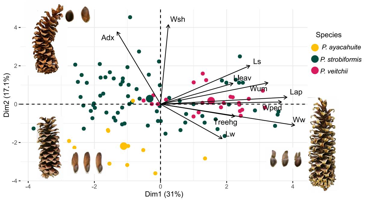
Figure 2 PCA of the 10 morphological characters measured in each individual. Dots in shades of green correspond to populations described as Pinus strobiformis, shades of blue correspond to populations described as Pinus veitchii and in red to Pinus ayacahuite.
The scatterplot between PC1 and PC2 shows individuals of the TMVB (identified as P. veitchii) are intermingled with individuals of P. strobiformis and are not intermediate with P. ayacahuite (Figure 2). Loading contributions for each variable can be seen in Table S6. The graphical representation of this pattern can be seen in the UPGMA dendrogram in Figure S3.
The Linear Discriminant Analysis explained 100 % of the variation of the original dataset (Figure 3). The variables with the highest discrimination coefficient from LD1 were needle sheath width (Wsh), seed length (Ls) and umbo width (Wum). The variables with the highest discrimination coefficients in LD2 were: needle length, seed wing width and tree height. The plot of LD1 vs. LD2 showed that individuals of P. strobiformis and P. veitchii, show significant overlap in the ordination space in a 95 % confidence (Figure 3). However, classification analysis through LDA with morphological characters showed that only 12.12 % in total individuals were misclassified, for example, of the 24 individuals of P. veitchii, only 5 were misclassified as P. strobiformis and 1 as P. ayacahuite (Table 2), while 7 % of individuals from P. strobiformis were classified as P. veitchii. All but one of the samples from P. ayacahuite were assigned correctly (90 %; Table 2).
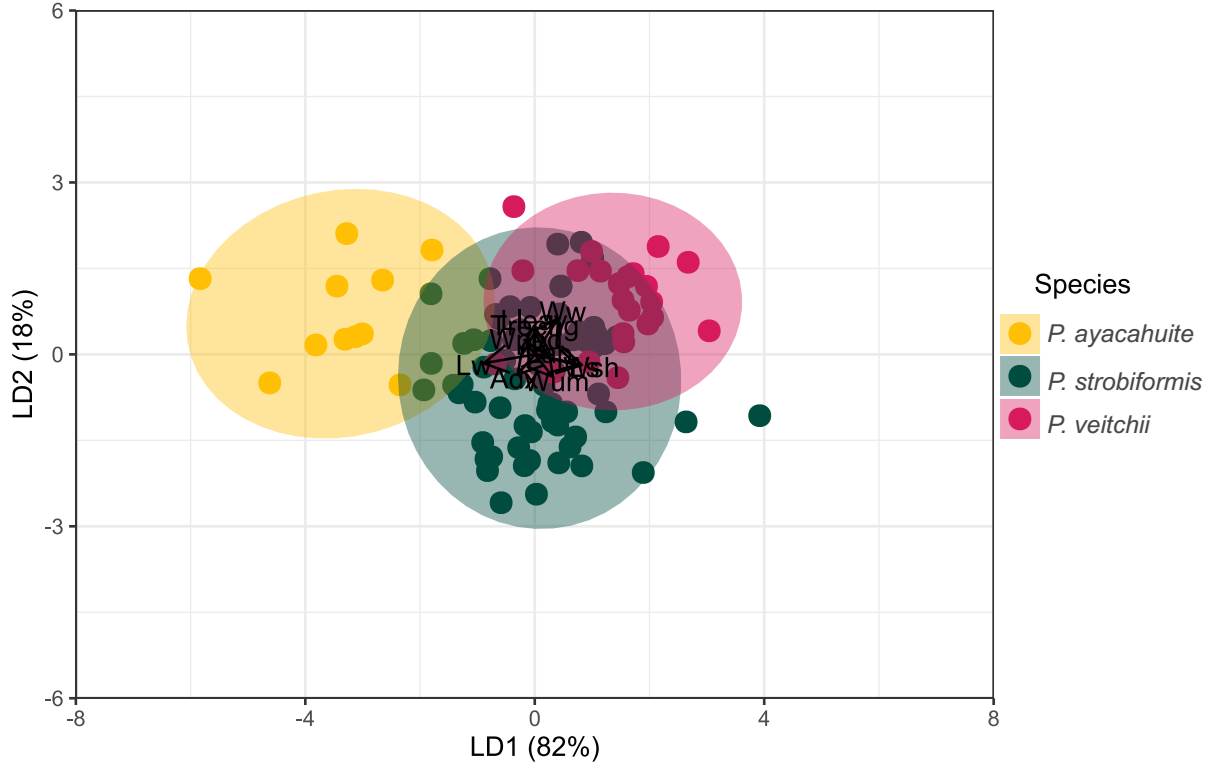
Figure 3 Plot of LD1 vs LD2 obtained from morphological variables from Pinus ayacahuite, Pinus strobiformis, and Pinus veitchii.
Table 2 Classification analysis of all the individuals in this study, based on LDA results.
| Predicted class (%) | |||
|---|---|---|---|
| Real class | P. strobiformis | P. veitchii | P. ayacahuite |
| P. strobiformis | 60 (93 | 5 (7) | 0 |
| P. veitchii | 5 (21 | 18 (75) | 1 (4) |
| P. ayacahuite | 1 (10 | 0 | 9 (90) |
Ecological niche models and environmental differentiation. The one-way ANOVA of the retained environmental variables found highly significant (P < = 0.01) differences among species for 9 variables: mean diurnal range (Bio2), isothermality (Bio3), maximum temperature of the warmest month (Bio5), mean temperature of the driest quarter (Bio9), precipitation of the warmest quarter (Bio18), precipitation of the coldest quarter (Bio19). Precipitation seasonality (Bio15) was moderately significant (P = 0.015) and precipitation of the driest month was not significant (Table S7). In the PCA the first component (PC1) explains 32.6 % of the variance, PC2 the 27.9 % of variance. No clear differentiation among groups was observed (Figure S4).
The ENM for the three taxa were better than expected by chance and had AUC values > 1 The best models selected with the AIC were Linear with a RM of 0.5 for P. veitchii, LQHP with a RM of 1.5 for P. strobiformis and Hinge with a RM of 1.5 for P. ayacahuite. The ENMs for P. strobiformis and P. ayacahuite had overprediction but were restricted mostly within their known distribution. The model with more overprediction was P. veitchii, with a predicted range across most of the TMVB where it only grown in a few isolated populations (Figure 4). The most important environmental variable was isothermality for all three species but in different proportions: P. strobiformis (37.9 %), P. veitchii (49.8 %) and P. ayacahuite (73.3 %). Another variable which was relevant for P. veitchii was Temperature annual range (9.5 %), but was not important for P. strobiformis nor P. ayacahuite. For P. strobiformis, the second most important variable was Maximum Temperature of the Warmest Month (17.5 %), and Precipitation of Coldest Quarter (7.8 %) and for P. ayacahuite: Annual Mean Temperature (16.1 %) and Precipitation Seasonality (2.6 %), see supplementary material (Table S8). The niche overlap tests (Hellinger’s I and Schoener’s D) show niche conservatism for most comparisons, with observed values being higher than expected by chance (Figure 5).
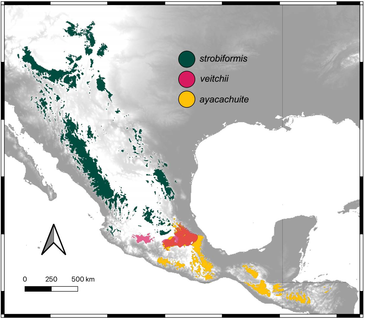
Figure 4 Climatic niche models for the present conditions for Pinus strobiformis, Pinus veitchii, and Pinus ayacahuite.
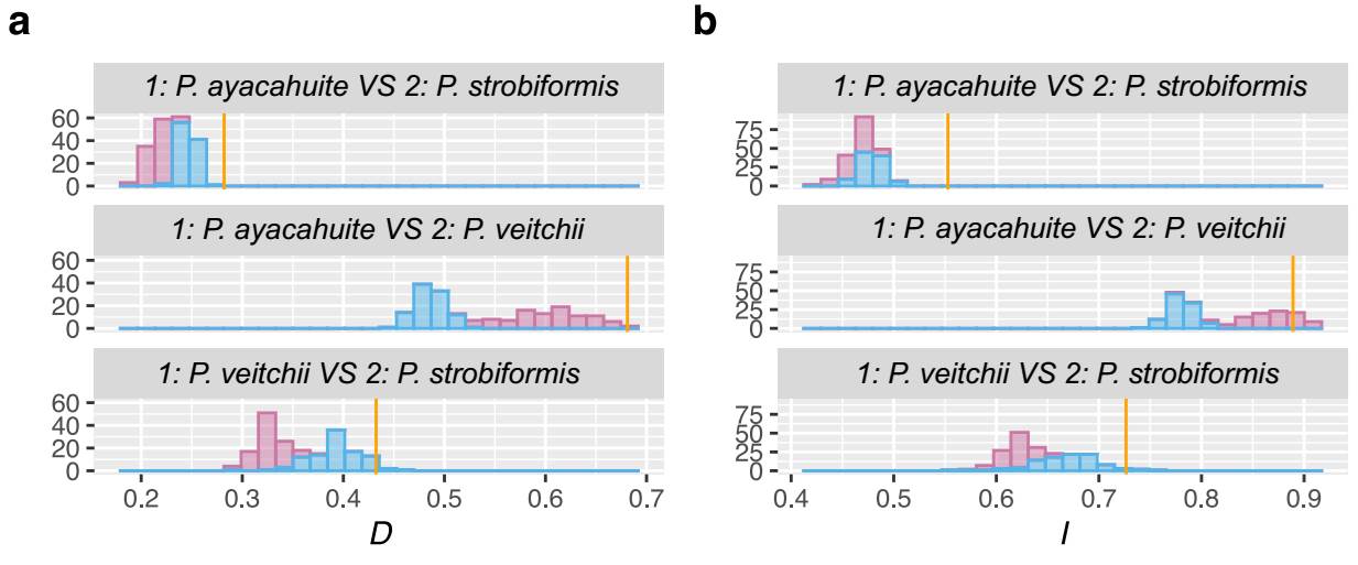
Figure 5 Background test results for the Pinus strobiformis-Pinus veitchii-Pinus ayacahuite species complex. The observed I and D values are shown by the yellow bars. The null distributions of a) D and b) I values are shown by the histograms.
Genetic analyses. The genetic clustering analyses showed a differentiation among all species. In all cases, P. strobiformis has recovered as differentiated genetic group (Figure 6A-C), while P. veitchii and P. ayacahuite showed some degree of overlap (Figure 6A-B) or admixture (Figure 6C). In particular, the admixture analyses showed no differentiation between P. ayacahuite and P. veitchii with K = 2, but the genetic structure was later recovered with higher K values, but with a pattern that can be interpreted as either introgression or incomplete lineage sorting (Figure 6C).
Discussion
Species delimitation and integrative taxonomy. There are several factors which make species delimitation difficult for white pine species of the TMVB. First, the wide distribution along a latitudinal cline of the P. strobiformis-P. veitchii-P. ayacahuite species complex provides a gradual transition of environmental conditions, instead of abrupt geographical barriers. Second, the high morphological variation in P. strobiformis could be due to environmental or underlying genetic factors such as local adaptation (Menon et al. 2018, Leal-Sáenz et al. 2020), or an interaction of both. This lack of clear limits makes it important to use a wide arrange of traits that represent the geographical variation of the species complex to be able to adequately identify independent lineages (De Queiroz 2007, Cicero et al. 2021).
Morphological traits showed significant differences among all taxa (ANOVA, MANOVA, MANCOVA, Tables S3-S5), but the PCA and LDA analyses do not show a clear-cut difference between P. veitchii and P. strobiformis (Figures 2 and 3). However, P. ayacahuite is morphologically distinct from the other two taxa. Contrary to our expectations, P. veitchii did not have intermediate morphological values, despite having an intermediate distribution and being in a potential contact zone. In other pine populations with known hybrid origins, the hybrids often exhibit intermediate morphological values between the parental species, as it has been described in P. densata Masters (Xing et al. 2014), hybrids between P. montezumae Lamb. and P. pseudostrobus Endl. (Delgado et al. 2007). In the latter case, hybrids were not consistently assigned to a hybrid cluster with a LDA but were also assigned to their parental species with nearly equal proportions. A similar case has been observed in a hybrid zone between P. echinata Hort. ex Carrière and P. taeda L., where hybrids were assigned with parental species in high proportion (Chen et al. 2004). However, with P. veitchii, only 12.5 % of individuals were assigned to P. strobiformis (Table 2).
Taxonomic treaties of white pines have classified P. veitchii as a variety of P. ayacahuite (Farjon 1998, Maya 2006, Leal-Sáenz et al. 2020), but Frankis (2009) observed that individuals from the TMVB had seeds and wings 5 to 10 times larger than those of P. ayacahuite, making it more similar to P. strobiformis, which is consistent with our results. Meanwhile, Businský (2008) has proposed that those populations should be seen as a separate species, P. veitchii.
Environmental differentiation. The ecological niche models recovered the known distribution for two of the three taxa. The exception was P. veitchii, which is known from just a few localities but has a much wider potential distribution (Figure 4). This could be due to historical or ecological reasons (barriers to dispersal, competition), or due to a higher uncertainty of the models when training with few presence points, leading to overprediction. The environmental variable that is more important for all taxa is isothermality, which is a consequence of the latitudinal cline of the species complex. The higher values of isothermality were seen in P. ayacahuite, consistent with a more tropical distribution (Del Castillo et al. 2004).
The one-way ANOVA showed a significant differentiation of most variables (the exception was Bio14 Precipitation in the driest month, Table S7) for the species complex, however, the PCA results show clinal variation rather than clearly defined clusters (Figure S4). All taxa exhibit overlapped in the environmental space, with P. veitchii displaying intermediate values. This result is the opposite of what was observed with morphology, where P. veitchii was not intermediate, but overlapped with P. strobiformis (Figure 4). This result was to be expected due to the geographically intermediate position of P. veitchii along a latitudinal cline, but contradicts the clear differentiation between P. veitchii and P. ayacahuite observed with morphological characters.
The lack of clear clustering in the PCA of environmental variables can be observed in the background test, where all comparisons are either no different to a random distribution or more similar than expected by chance (Figure 5). This result coincides with previous studies where P. strobiformis and P. ayacahuite are significantly more similar than expected by chance (Moreno-Letelier et al. 2013, Aguirre-Gutiérrez et al. 2015). However, as these two taxa are not sister species, the niche conservatism can be explained by shared ancestry and evolution in allopatry (McCormack et al. 2009). The case of P. veitchii requires more study as it has nested niche with P. strobiformis and P. ayacahuite (Figure 5) which may hint of incipient peripatric speciation (Moreno-Letelier & Piñero 2009, Moreno-Letelier et al. 2013, Castellanos-Morales et al. 2016).
Finally, the lack of niche divergence in the three species constitutes evidence against the possibility of a hybrid origin of P. veitchii, because in the absence of other reproductive barriers, different environments would prevent back-crossings. The well documented case of hybrid speciation in pines, Pinus densata, exhibits significant ecological niche differentiation of the hybrid and parental species, which in turn reinforced the reproductive barriers (Mao & Wang 2011). However, partially overlapping ecological niche observed in Mexican white pines is more suggestive of allopatric and/or peripatric speciation (McCormack et al. 2009).
Genetic analyses. The genetic analyses showed an opposite pattern to that observed with morphological characters. Our results show a closer relationship between P. veitchii and P. ayacahuite (Figure 6A-C), and a clear differentiation of P. strobiormis. However, there is evidence that introgression might have played a role in those similarities. The PCA analysis has an area of overlap between P. ayacahuite and P. veitchii (Figure 6A), which can be later seen as evidence of gene flow between those two species in the admixture analyses (Figure 6C). However, standard genetic aggregation analyses cannot determine the direction or the age of said gene flow. Therefore, we require further analyses to be able to clarify how speciation occurred and whether the genetic similarities are due to introgression after speciation or are the result of incomplete lineage sorting (Zhou et al. 2016).
Integrative taxonomy. As mentioned above, integrative taxonomy aims at including multiple lines of evidence for species delimitation (Dayrat 2005). In this study we used the Unified Species Complex (De Queiroz 2007) in order to aid us in this task. Our results show two lines of evidence supporting the existence of three independent lineages: morphology and genetic differentiation (Figure 7), while niche divergence was not conclusive. However, De Queiroz (2007) stated that under the unified species concept the presence of a specific property that separates a lineage is evidence (morphology and genetic structure in our case), while the absence of a property (niche divergence) only means that the lineage has not evolved that property, but it is not evidence against independence.
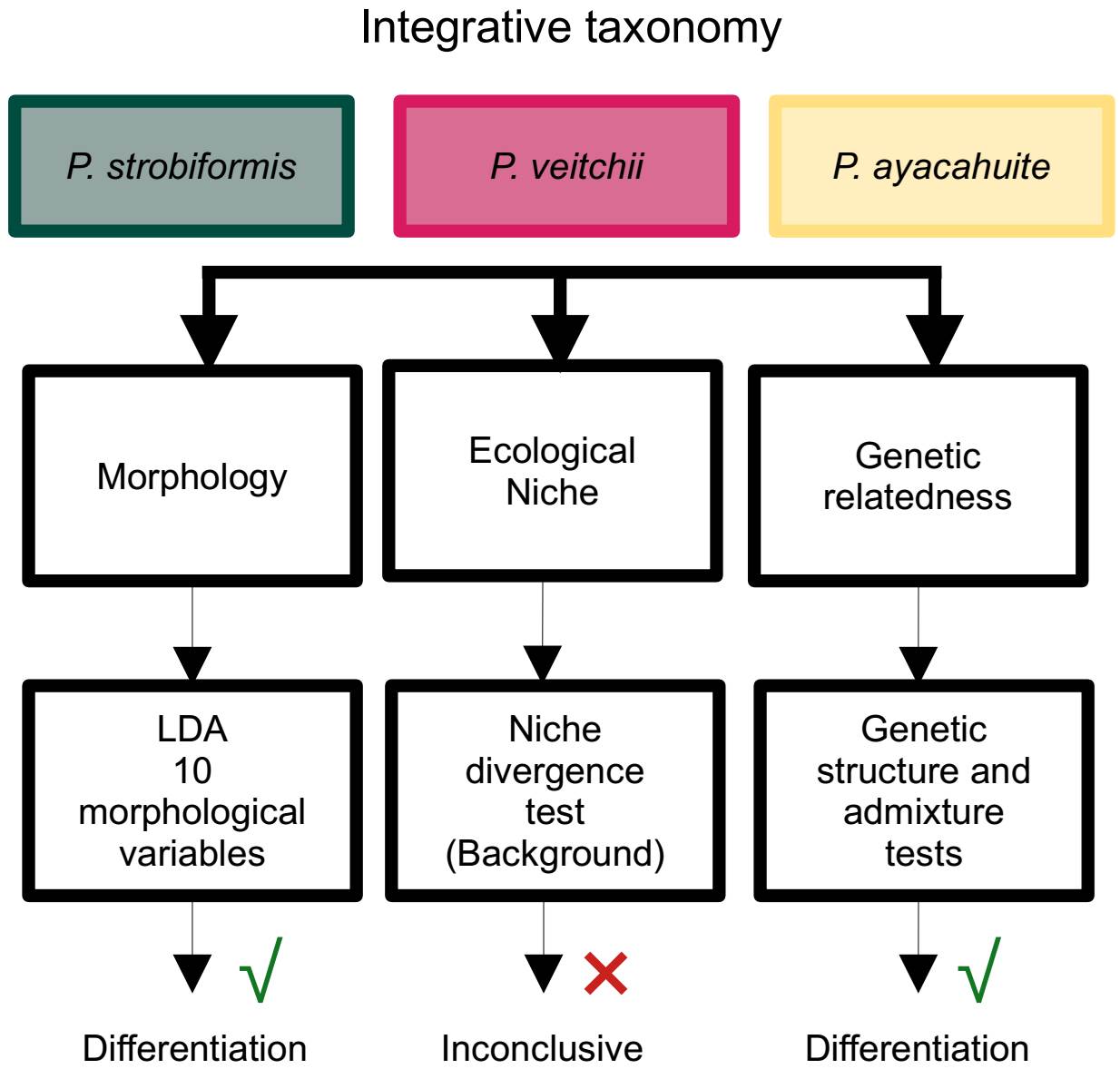
Figure 7 Summary of the process of species delimitation using integrative taxonomy and a Unified Species Concept (De Queiroz 2007).
The P. strobiformis-P. veitchii-P. ayacahuite species complex from a latitudinal cline, going from the Southwestern United States to El Salvador (Lanner 1996). The TMVB, is where the Southern limit of P. strobiformis meets with the Northern limit of P. ayacahuite. This area has been identified as a biological corridor (Ornelas et al. 2013, Mastretta-Yanes et al. 2015) and important for hybridization in several species (Delgado et al. 2007, López-Reyes et al. 2015). The combined evidence of our study shows that P. vetichii, P. strobiformis and P. ayacahuite constitute independent lineages, which could be considered species in their own right, supporting our hypothesis. However, out results do not support the hybrid origin of P. veitchii, because neither the morphological nor genetic analyses show intermediate values, as it has been observed in other pine populations with known hybrid origins (Delgado et al. 2007). The genetic information shows a clear differentiation between P. strobiformis and P. veitchii, with evidence of introgression with P. ayacahuite. Therefore, more analyses are required to be able to distinguish between introgression and shared ancestral polymorphism and determine which taxon is the sister species to P. vetichii (Zhou et al. 2016, Montes et al. 2022). We did not identify significant ecological differentiation; however, it is not a requirement to recognize a species under the unified species concept (De Queiroz 2007).
Supplementary material
Supplemental material for this article can be accessed here https://doi.org/10.17129/botsci.3364.


 nueva página del texto (beta)


