


 text new page (beta)
 Article in xml format
 Article references
 Send this article by e-mail
 Cited by SciELO
  Similars in
SciELO
Similars in
SciELO 
 Permalink
1. Introduction
Since the 1960s, following the Prebisch-Singer hypothesis of terms of trade deterioration, policymakers in developing countries have been aiming to increase the variety of goods that they export. Several Asian countries such as South Korea and Taiwan are examples of remarkable export-led growth. Some economists have found an association between the degree of export diversification and economic growth. For example, Sachs and Warner (1995) suggest a correlation between low export diversification and slow growth.1 However, despite the desire of policymakers to increase the variety of exported goods, until recently trade economists had not paid much attention to this issue, mainly because classical trade theories focus on the advantages of specialization into products in which countries have comparative advantages rather than diversification or increasing the variety of export goods.2
However, the theoretical contribution by Melitz (2003) triggered a rapid increase in research on export diversification. His model is referred to in the literature as the heterogeneous firms trade model. It shows that a reduction in trade barriers allows an initially nonexporting firm to become an exporter. Melitz (2003) also incorporated firm heterogeneity into Krugman’s (1980) model of trade under increasing returns and monopolistic competition. Firms differ in their levels of productivity and thus their marginal costs, while they also incur sales-related costs in both domestic and export markets. Such sales-related costs are assumed to be higher for export markets than for domestic markets.
Firms that have sufficiently high productivity levels can thus absorb export-related costs and can be active in both domestic and export markets. By contrast, firms that have low levels of productivity cannot be active even in domestic markets, while those that have medium levels serve only the domestic market. The borders among these three types of firms are determined by two cut-off productivity conditions.
This paper focuses on the case of Mexico, which has undergone a series of large-scale trade liberalization activities culminating in the formation of NAFTA. Despite the apparent positive effect of NAFTA on the Mexican economy shortly after its formation (Lederman, Maloney and Serven, 2004, offered a generally positive assessment of NAFTA’s effect on the Mexican economy), economic performance over the past decade in Mexico has remained “lacklustre, trailing that of many other developing nations” (Hanson, 2010: 2). It is thus worth revisiting NAFTA’s impact on the Mexican economy. Specifically, this paper focuses on the change in the variety of Mexico’s export goods.
The contributions of this paper are threefold. First, it shows the trends in the goods exported to major US trade partners. Second, it uses disaggregated trade data to find that Mexico’s unilateral trade liberalization has increased the possibility of any particular good being exported. Third, it points out a potential problem when selecting a comparison country for the computation of the variety index (Feenstra and Kee, 2007) and thus proposes a variety index with a multi-county base. It then carries out an econometric analysis using this improved version and shows that NAFTA is not associated with an increase in the variety index, which is at odds with the findings presented in the literature.
One of the early papers related to the topic of this paper was Helpman, Melitz and Rubinstein (2008), which developed a theorybased gravity model of trade that predicts positive as well as zero trade flows across pairs of countries. Using total trade value data for 158 countries in 1986, this paper showed that among 24 806 possible bilateral export relationships, only 11 146 pairs have non-zero exports. More importantly, it found that the usual gravity equation variables also affect the probability of the occurrence of a bilateral export relationship.
While Helpman, Melitz and Rubinstein (2008) studied the export relationships between country pairs, others have examined the extensive margins or trade value generated by the sale of new goods. Kehoe and Ruhl (2009), for example, analyzed the relation between trade liberalization and extensive margins and find an overall positive association. This paper studied NAFTA, but did not conduct an econometric analysis to explain its effects. Moreover, its analysis of the Mexico-US trade agreement used data from 1989, five years before the formation of NAFTA. Baier, Bergstran and Feng (2011) employed a panel econometric methodology to examine the effects of economic integration agreements on aggregate trade flows using a gravity equation model and finds economically and statistically significant effects on both intensive and extensive margins. Feenstra and Kee (2007) proposed an index for export variety and found a positive association between NAFTA membership and an increase in the export variety index.
Our paper departs from the literature in three aspects. First, unlike the studies mentioned above, we use raw disaggregated data to identify increases in the number of product categories exported. Second, we acknowledge a potential problem in the selection of a comparison base (Feenstra and Kee, 2007) and propose a revised version of the index. Finally, econometric analysis we present shows that NAFTA is not associated with an increase in the variety index.
Section 2 describes the evolution of zeros. Section 3 presents the econometric analyses using raw disaggregated data. The variety index is discussed in section 4. The final section concludes.
2. The evolution of zeros
Recent studies of the exports of new goods show a very large number of zeros in the world trade matrix. According to Baldwin and Harrigan, “the United States imported in nearly 17 000 different 10-digit HS categories from 228 countries, for a total of over 3.8 million potential trade flows. Over 90% of these potential trade flows are zeros” (2011: 72). Hummels and Klenow (2005) further showed that 60 percent of the greater export of larger economies in their sample of 126 countries is due to the increase of the number of exported products.
Mexico was the third largest import partner for the US in the period 1989-2006. For Mexico, the US is by far its largest trade partner both for imports and for exports. The share of the US in Mexico’s exports has steadily increased and reached 89% in 2006. We analyze Mexico’s exports using US import data since they are available at the most disaggregated level of classification, namely 10-digit HS codes. The data come from Feenstra and Kee (2004) and cover the years 1989 to 2006.3 The 10-digit HS codes during this period cover, in total, 24 818 items.4 Table 1 shows the evolution of the number of zeros in US imports from its top 20 import partners plus Colombia and Chile, from 1989 to 2006.
Table 1 The number of zeros in US imports from the 20 largest import partners plus Colombia and Chile: 1989-2006
| Year | Canada | Japan | Mexico | China | Germany | Taiwan | United Kingdom | |
| 1989 | 15179 | 15748 | 19105 | 19198 | 15600 | 17859 | 15884 | |
| 1990 | 14931 | 15673 | 19124 | 18918 | 15481 | 17926 | 15848 | |
| 1991 | 14756 | 15516 | 19043 | 18634 | 15401 | 17947 | 15733 | |
| 1992 | 14678 | 15721 | 18994 | 18272 | 15467 | 18049 | 15731 | |
| 1993 | 14461 | 15726 | 18761 | 17842 | 15357 | 17932 | 15463 | |
| 1994 | 13907 | 15370 | 18084 | 17254 | 14876 | 17690 | 15033 | |
| 1995 | 13484 | 15377 | 17176 | 16925 | 14743 | 17608 | 14839 | |
| 1996 | 13260 | 15211 | 16478 | 16555 | 14531 | 17410 | 14475 | |
| 1997 | 12729 | 14826 | 15980 | 15793 | 14020 | 16949 | 13992 | |
| 1998 | 12990 | 15072 | 16245 | 15578 | 14283 | 17141 | 14175 | |
| 1999 | 12922 | 15065 | 16161 | 15160 | 14280 | 17103 | 14382 | |
| 2000 | 12847 | 15076 | 16117 | 14621 | 14104 | 16950 | 14272 | |
| 2001 | 13010 | 15292 | 16250 | 14506 | 14201 | 17077 | 14503 | |
| 2002 | 12724 | 15180 | 16105 | 13769 | 13991 | 16898 | 14443 | |
| 2003 | 12844 | 15157 | 16203 | 13379 | 14054 | 16856 | 14546 | |
| 2004 | 12920 | 15126 | 16095 | 12837 | 13987 | 16724 | 14460 | |
| 2005 | 12912 | 14986 | 16009 | 12126 | 14078 | 16741 | 14640 | |
| 2006 | 12959 | 14892 | 15993 | 11691 | 14017 | 16746 | 14672 | |
| Change, 1989-2006 | -2220 | -856 | -3112 | -7507 | -1583 | -1113 | -1212 | |
| Year | Korea | France | Italy | Singapore | Malasya | Thailand | Venezuela | |
| 1989 | 18954 | 16601 | 16809 | 22163 | 22982 | 21904 | 23453 | |
| 1990 | 19061 | 16597 | 16745 | 22199 | 22846 | 21777 | 23078 | |
| 1991 | 19320 | 16585 | 16643 | 22185 | 22651 | 21636 | 23347 | |
| 1992 | 19410 | 16637 | 16676 | 22167 | 22489 | 21396 | 23505 | |
| 1993 | 19229 | 16384 | 16376 | 22083 | 22286 | 21110 | 23446 | |
| 1994 | 18903 | 15895 | 15823 | 21928 | 22052 | 20850 | 23390 | |
| 1995 | 18737 | 15705 | 15594 | 21910 | 21937 | 20692 | 23533 | |
| 1996 | 18725 | 15439 | 15249 | 21943 | 21843 | 20690 | 23348 | |
| 1997 | 18283 | 15000 | 14714 | 21611 | 21682 | 20508 | 23289 | |
| 1998 | 17853 | 15140 | 14924 | 21670 | 21603 | 20341 | 23411 | |
| 1999 | 17516 | 15116 | 14941 | 21627 | 21601 | 20182 | 23454 | |
| 2000 | 17474 | 14959 | 14611 | 21575 | 21391 | 19957 | 23432 | |
| 2001 | 17489 | 15026 | 14764 | 21765 | 21493 | 20005 | 23396 | |
| 2002 | 17143 | 15041 | 14460 | 21699 | 21417 | 19794 | 23398 | |
| 2003 | 17246 | 15040 | 14525 | 21670 | 21404 | 19675 | 23432 | |
| 2004 | 17069 | 15053 | 14457 | 21703 | 21228 | 19488 | 23438 | |
| 2005 | 16850 | 15126 | 14424 | 21643 | 21073 | 19302 | 23480 | |
| 2006 | 16938 | 15096 | 14270 | 21463 | 20933 | 19149 | 23681 | |
| Change, 1989-2006 | -2016 | -1505 | -2539 | -700 | -2049 | -2755 | 228 | |
| Year | Hong Kong | Brazil | Saudi Arabia | Philippines | Switzerland | Indonesia | Colombia | Chile |
| 1989 | 19379 | 20897 | 24589 | 22349 | 19139 | 23208 | 23362 | 23676 |
| 1990 | 19468 | 21122 | 24629 | 22422 | 19170 | 23061 | 23211 | 23687 |
| 1991 | 19481 | 21127 | 24627 | 22400 | 19229 | 22914 | 23053 | 23677 |
| 1992 | 19600 | 21044 | 24559 | 22309 | 19265 | 22688 | 23031 | 23678 |
| 1993 | 19574 | 20951 | 24542 | 22235 | 19150 | 22309 | 23034 | 23737 |
| 1994 | 19473 | 20678 | 24522 | 22051 | 18748 | 22190 | 22967 | 23627 |
| 1995 | 19384 | 20860 | 24444 | 21935 | 18573 | 21978 | 23048 | 23642 |
| 1996 | 19395 | 20859 | 24436 | 21878 | 18413 | 21771 | 23013 | 23625 |
| 1997 | 19196 | 20829 | 24374 | 21756 | 17944 | 21483 | 22927 | 23602 |
| 1998 | 19480 | 20932 | 24279 | 21670 | 18158 | 21313 | 22961 | 23555 |
| 1999 | 19569 | 20646 | 24288 | 21654 | 18287 | 21223 | 22732 | 23495 |
| 2000 | 19351 | 20146 | 24171 | 21519 | 18131 | 21118 | 22490 | 23475 |
| 2001 | 19517 | 20076 | 24165 | 21562 | 18287 | 21128 | 22436 | 23395 |
| 2002 | 19347 | 19614 | 24241 | 21496 | 18346 | 21011 | 22237 | 23249 |
| 2003 | 19257 | 19234 | 24299 | 21457 | 18435 | 20979 | 22017 | 23119 |
| 2004 | 19238 | 18963 | 24263 | 21431 | 18414 | 20906 | 21911 | 23112 |
| 2005 | 19032 | 18846 | 24246 | 21388 | 18377 | 20718 | 21723 | 23002 |
| 2006 | 18924 | 18775 | 24228 | 21223 | 18305 | 20568 | 21735 | 23030 |
| Change, 1989-2006 | -455 | -2122 | -361 | -1126 | -834 | -2640 | -1627 | -646 |
Source: Author’s calculation based on US imports data at HS 10 digit level.
The order of the countries in the table represents the ranking of exports into the US over this period, except Colombia (ranked 29) and Chile (ranked40).5 Mexico ranks number three following Canada and Japan. There were 19 105 zeros in 1989, which decreased to 15 993 in 2006. The last row in Table 1 shows the reduction in zeros during the investigated period. The number for Mexico (-3112) is second only to China, a huge country that is rapidly and dramatically increasing its exports across the world. In this sense, China can be considered to be an exceptional case. Mexico had more zeros, or non-exported items, than Korea and Taiwan in 1989. In 2006, the opposite was true. In other words, Mexico has surpassed Korea and Taiwan in terms of the variety of its exports to the US, and is close to the level of France.
However, it is important to seek data from well before 1986 in order to assess the evolution in the number of exported goods during Mexico’s unilateral trade liberalization from 1986 and during the formation of NAFTA from 1994. Although the 10-digit HS data are only available from 1989, US trade data (with a trade statistics seven-digit code) are available from 1972 to 1988. Table 2 shows the evolution of zeros for 1972-1988. The decrease in the number of zeros for Mexico is lower than for the other major US import partners during this period. China registers the largest decrease in the number of zeros, but this decrease is less impressive than the decrease it obtained during the 1989-2006 period.
Table 2 The number of zeros in US imports from the 20 largest import partners plus Colombia and Chile: 1972-1988
| Year | Canada | Japan | Mexico | China | Germany | Taiwan | United Kingdom | |
| 1972 | 19892 | 19404 | 21911 | 23247 | 19757 | 21844 | 19665 | |
| 1973 | 19681 | 19606 | 21669 | 23153 | 19709 | 21816 | 19514 | |
| 1974 | 19506 | 19521 | 21390 | 23031 | 19675 | 21725 | 19510 | |
| 1975 | 19548 | 19482 | 21485 | 22905 | 19745 | 21546 | 19613 | |
| 1976 | 19435 | 19236 | 21414 | 22696 | 19505 | 21201 | 19413 | |
| 1977 | 19512 | 19344 | 21510 | 22791 | 19627 | 21356 | 19486 | |
| 1978 | 18379 | 18411 | 20708 | 22515 | 18589 | 20488 | 18450 | |
| 1979 | 18305 | 18388 | 20711 | 22303 | 18608 | 20387 | 18442 | |
| 1980 | 17906 | 17978 | 20707 | 21736 | 18146 | 20125 | 18137 | |
| 1981 | 17686 | 17852 | 20705 | 21312 | 18019 | 19922 | 18084 | |
| 1982 | 17551 | 17514 | 20670 | 21071 | 17855 | 19536 | 18008 | |
| 1983 | 17469 | 17173 | 20203 | 20855 | 17485 | 19190 | 17768 | |
| 1984 | 17041 | 16570 | 19953 | 20511 | 17045 | 18716 | 17123 | |
| 1985 | 16532 | 15217 | 19981 | 19719 | 16054 | 17736 | 16199 | |
| 1986 | 16544 | 15490 | 19744 | 19593 | 16125 | 17882 | 16425 | |
| 1987 | 16422 | 15960 | 19441 | 19383 | 16328 | 17935 | 16438 | |
| 1988 | 16359 | 16352 | 19377 | 19199 | 16481 | 18110 | 16710 | |
| -3533 | -3052 | -2534 | -4048 | -3276 | -3734 | -2955 | ||
| Year | Korea | France | Italy | Singapore | Malasya | Thailand | Venezuela | |
| 1972 | 22682 | 20321 | 20456 | 23372 | 23637 | 23501 | 23631 | |
| 1973 | 22572 | 20218 | 20469 | 23291 | 23584 | 23396 | 23608 | |
| 1974 | 22356 | 20188 | 20449 | 23208 | 23580 | 23317 | 23548 | |
| 1975 | 22179 | 20170 | 20411 | 23173 | 23519 | 23315 | 23620 | |
| 1976 | 21798 | 20031 | 20271 | 23057 | 23434 | 23168 | 23635 | |
| 1977 | 21852 | 20194 | 20406 | 23152 | 23453 | 23139 | 23710 | |
| 1978 | 21249 | 19145 | 19420 | 22745 | 23271 | 22936 | 23669 | |
| 1979 | 21386 | 19155 | 19403 | 22659 | 23189 | 22880 | 23657 | |
| 1980 | 21199 | 18936 | 19292 | 22550 | 23178 | 22798 | 23603 | |
| 1981 | 20914 | 18682 | 19003 | 22404 | 23097 | 22655 | 23597 | |
| 1982 | 20680 | 18510 | 18751 | 22346 | 23117 | 22511 | 23570 | |
| 1983 | 20393 | 18169 | 18375 | 22270 | 23003 | 22459 | 23407 | |
| 1984 | 19919 | 17571 | 17824 | 22075 | 22841 | 22191 | 23302 | |
| 1985 | 19135 | 16410 | 16183 | 21756 | 22521 | 21794 | 23302 | |
| 1986 | 19048 | 16523 | 16476 | 21750 | 22548 | 21859 | 22964 | |
| 1987 | 18953 | 16913 | 16871 | 21763 | 22462 | 21759 | 23007 | |
| 1988 | 18977 | 17095 | 17058 | 21753 | 22443 | 21632 | 23026 | |
| -3705 | -3226 | -3398 | -1619 | -1194 | -1869 | -605 | ||
| Year | Hong Kong | Brazil | Saudi Arabia | Philippines | Switzerland | Indonesia | Colombia | Chile |
| 1972 | 21631 | 22831 | 23915 | 23231 | 21450 | 23765 | 23203 | 23818 |
| 1973 | 21633 | 22547 | 23923 | 23092 | 21474 | 23738 | 23132 | 23842 |
| 1974 | 21626 | 22534 | 23915 | 22984 | 21383 | 23686 | 23061 | 23798 |
| 1975 | 21505 | 22589 | 23914 | 22979 | 21483 | 23635 | 23088 | 23748 |
| 1976 | 21199 | 22593 | 23921 | 22827 | 21322 | 23593 | 23004 | 23632 |
| 1977 | 21384 | 22640 | 23916 | 22840 | 21471 | 23579 | 23178 | 23667 |
| 1978 | 20653 | 22202 | 23906 | 22451 | 20789 | 23473 | 23069 | 23581 |
| 1979 | 20669 | 22131 | 23884 | 22438 | 20793 | 23377 | 23175 | 23570 |
| 1980 | 20516 | 22121 | 23870 | 22403 | 20574 | 23396 | 23140 | 23600 |
| 1981 | 20315 | 21818 | 23827 | 22255 | 20415 | 23269 | 23187 | 23615 |
| 1982 | 20133 | 21678 | 23800 | 22224 | 20297 | 23213 | 23218 | 23589 |
| 1983 | 20003 | 21364 | 23776 | 22210 | 20008 | 23225 | 23137 | 23454 |
| 1984 | 19562 | 20558 | 23735 | 22001 | 19624 | 23038 | 22987 | 23370 |
| 1985 | 18285 | 20210 | 23674 | 21580 | 19124 | 22561 | 22844 | 23331 |
| 1986 | 18577 | 20471 | 23636 | 21728 | 18994 | 22732 | 22840 | 23101 |
| 1987 | 18784 | 20699 | 23728 | 21748 | 19028 | 22629 | 22717 | 23036 |
| 1988 | 19069 | 20623 | 23752 | 21779 | 19232 | 22558 | 22636 | 22888 |
| -2562 | -2208 | -163 | -1452 | -2218 | -1207 | -567 | -930 |
Source: Author’s calculation based on US imports data at HS 10 digit level
Since the absolute level of the number of zeros in the initial year of each of the time series (i.e., 1989 and 1972, respectively) varies by country, we indexed the number of zeros by taking 1989 as the base year for the 1989-2006 period and 1988 as the base year for the 1972-1988 period in order to permit comparison. The result is shown in Figure 4.6 Imports from China underwent the largest decrease in this zero index, while Canada also displayed a steady and rapid decrease in the index. The decrease in the index of Mexico from the 1970s to the first half of the 1980s was modest compared with the other major US trade partners, but it accelerated from around 1985 to 1997 and retained this higher rate of decrease thereafter. Although the US HS 10-digit trade data at from the Center for International Data at UC Davis are available only up to 2006, the number of zeros between 2006 and 2012 may give some useful information, especially because of the crisis in 2008-2009 and subsequent recovery.
Thus Figure 5 shows the zero index (using 1991 as the base year) of US imports from its major import partners at HS 6-digit level from 1991 to 2012. There is a clear rise in the number of zeros during the crisis and some recovery after the crisis. This may indicate that business cycles have a stronger effect on trade flows than do trade agreements such as NAFTA.7 To see the potential effects of economic downturn during the crisis from the side of Mexico’s export, Figure 6 shows the zero index of Mexico’s exports at HS 6-digit to its major markets.8 As in the previous case, the zero index rose in the crisis period, especially for the developed countries, notably the US, which were bitterly hit by the crisis.
3. Econometric analysis using raw trade data
This section performs an econometric analysis using raw trade data to examine whether the probability of a particular product being exported is associated with Mexico’s periods of trade liberalization. As noted in the previous section, it is imperative to use trade data from a sufficiently long period of time before 1986 in order to appropriately capture the effects of the two major series of Mexico’s trade liberalization: the unilateral trade liberalization from 1986 and inception of NAFTA from 1994. It is logically straightforward to assume that NAFTA may have had a positive impact on Mexico’s export variety because the US eliminated its import tariffs on Mexican goods. On the other hand, Mexico’s unilateral trade liberalization was an initiative on the side of Mexico to reduce its import tariffs, and thus did not directly work to reduce its trade partners’import tariffs. However, this initiative may have increased Mexico’s export diversification through two channels.
The first channel is due to better access to affordable inputs, which may eventually have led to an increase of export variety. Indeed, the Mexican government’s first action in its series of unilateral trade liberalization was the elimination of license requirements, official import prices, and quantitative restrictions, in order to improve Mexican products competitiveness.9 The other is Mexico’s accession to the General Agreement on Tariffs and Trade (GATT) in 1987, which itself was made possible by Mexico’s unilateral trade liberalization in 1986. We use five-digit SITC trade data, which are the only data available with consistent product codes for a sufficiently long period.10 We use Mexico’s export data on the 50 largest export destinations at the five-digit SITC level for the longest possible date range, namely 1962-2010. The following equation is then estimated using a Probit model:
where y takes 1 when the dependent variable (i.e., the trade value) takes a positive number, and 0 otherwise. x is the vector of explanatory variables, namely the GDP of destination countries; the distance between Mexico and destination countries; the NAFTA dummy, which takes 1 if the destination country is the US and the years are on or after 1994, and 0 otherwise; the Mexico unilateral liberalization dummy, which takes 1 if the years are on or after 1986; the common language dummy; and the dummies for years, destinations, and two-digit SITC codes.11 β ′ is the vector of parameters for these variables. φ (v) is a standard normal density function.
The summary statistics are in Table 3 and the estimation results are in Table 4. The large number of observations -more than 2 million- comes from 48 years times 50 partner countries times approximately 1000 SITC codes. The first column only includes the NAFTA dummy, while the second column includes both the NAFTA dummy and Mexico’s unilateral liberalization dummy. The variable of interest, NAFTA, shows negative and statistically highly significant coefficients, -0.147. Contrary to the sign of NAFTA, Mexico’s unilateral liberalization dummy shows a statistically significant positive coefficient with a relatively large magnitude, 0.781. Namely, this estimation result suggests that NAFTA is negatively associated with an increase in the probability of a particular product being exported while Mexico’s unilateral liberalization is positively associated. However, these results might have occurred because of the small change in the number of zeros after 2000, as shown in Table 1 and Figure 4. Thus, the same estimation was carried out for 1972-2001 as a robustness check (i.e., to make it comparable with the 1972-2001 study period of Feenstra and Kee, 2007).
Table 3 Summary statistics 1962-2010
| Variable | Observations | Mean | Standard deviation | Minimum | Maximum | Expected sign for coefficient estimate |
| Log of export value | 2218524 | 0.533 | 1.604 | 0 | 17.382 | Non-applicable |
| Log of GDP | 1956108 | 24.599 | 2.298 | 17.277 | 30.312 | Positive |
| Log of distance | 2218524 | 8.694 | 0.812 | 6.969 | 9.719 | Negative |
| Common language | 2218524 | 0.367 | 0.482 | 0 | 1 | Positive |
| NAFTA | 2218524 | 0.007 | 0.084 | 0 | 1 | Positive/Negative/Neutral |
| Mexico unilateral liberalization | 2218524 | 0.510 | 0.500 | 0 | 1 | Positive/Negative Neutral |
Table 4 Estimation results: Probit using five-digit SITC data for 1962-2010
| (1) | (2) | |
| Log of GDP | ||
| Log of distance | ||
| Common language | ||
| NAFTA | ||
| Mexico unilateral liberalization | ||
| Number of observations | 1 956 108 | 1 956 108 |
| Pseudo R-squared | 0.243 | 0.243 |
t statistics in parentheses *p< 0.05, **p < 0.01, ***p < 0.001.
The results in Table 5 still show the statistically significant negative coefficient estimate for the NAFTA dummy and the statistically significant positive coefficient estimate for Mexico’s unilateral liberalization dummy, although the magnitude is much attenuated in the latter. The smaller coefficient estimate for Mexico’s unilateral liberalization dummy during the shorter period of study (1972-2001) seems reasonable because the number of zero trade after 2002 declined only slightly, as is shown above, reducing the relative positive impact of the unilateral liberalization. Another issue which should be considered is that the US has always been the main destination of the Mexican exports. Therefore, Mexico’s unilateral liberalization might have coincided with tariff reduction of the US on Mexican products. Unfortunately, the US tariff data are available only from 1989, which hinders an econometric analysis. However, the duty amounts collected at the US custom office are available. Thus, as measures of the US average tariffs, we have computed the ratio of duties collected to dutiable imports and the ratio of duties collected to total imports.12 Figure 1 shows the US average tariffs across all import partners. The average tariffs are almost constant in the 1980s to the beginning of the 1990s. Figure 2 shows the ratio of duties collected to dutiable imports, while Figure 3 shows the ratio of duties collected to total imports by the US top 10 import partners. In both cases, the tariffs on Mexican products in the 1980s to the beginning of the 1990s are almost constant. Given this evidence, we can discard the possibility that the US tariff reduction on Mexican products was the real cause of the positive impact of Mexico’s unilateral trade liberalization documented above. These results contrast with previous findings of NAFTA’s positive association with diversification or an increase in the variety of Mexico’s exports. Because this effect might be different across sectors, the same estimation was carried out for the machinery sector, which typically has the largest trade values.13
Table 5 Estimation results: Probit using five-digit SITC data for 1972-2001
| (1) | (2) | |
| Log of GDP | ||
| Log of distance | ||
| Common language | ||
| NAFTA | ||
| Mexico unilateral liberalization | ||
| Number of observations | 1 191 960 | 1 191 960 |
| Pseudo R-squared | 0.230 | 0.230 |
t statistics in parentheses *p< 0.05, **p < 0.01, ***p < 0.001.
The estimation results in Table 6 (for products in machinery sector only) show the statistically significant negative coefficient for NAFTA dummy, -0.192, which is similar in its magnitude with the case in Table 4 (for products in all industries), -0.147, and also shows the statistically significant positive coefficient for Mexico’s unilateral liberalization, 0.818, which is close to 0.781 in Table 4. Table 7 (for 1972-2001) shows the coefficient estimates for NAFTA and Mexico’s unilateral liberalization with the expected signs and the smaller magnitude of Mexico’s unilateral liberalization, being consistent with the case of the products in all industries (Table 4 and Table 5). The other control variables have the expected signs, except for the distance variable in Table 6, which is probably caused by the rapid decrease of zero trade (higher incidence of a product being exported) with China and Chile, which are distant from Mexico, as can be seen in Figure 6.
Table 6 Estimation results: Probit for the machinery sector using five-digit SITC data for 1972-2010
| (1) | (2) | |
| Log of GDP | ||
| Log of distance | ||
| Common language | ||
| NAFTA | ||
| Mexico unilateral liberalization | ||
| Number of observations | 213 817 | 213 817 |
| Pseudo R-squared | 0.273 | 0.273 |
t statistics in parentheses *p< 0.05, **p < 0.01, ***p < 0.001.
Table 7 Estimation results: Probit for the machinery sector using five-digit SITC data for 1972-2001
| (1) | (2) | |
| Log of GDP | ||
| Log of distance | ||
| Common language | ||
| NAFTA | ||
| Mexico unilateral liberalization | ||
| Number of observations | 130 290 | 130 290 |
| Pseudo R-squared | 0.246 | 0.246 |
t statistics in parentheses *p< 0.05, **p < 0.01, ***p < 0.001.
3.1. Panel unit root tests
When estimating a gravity model using panel data, there is a potential problem caused by nonstationarity (Quah, 1994). Zwinkels and Beugelsdijk (2010) point out the lack of treatment for nonstationarity in the gravity model literature and argue that ignoring nonstationarity can lead to overestimated coefficients. Thus, we performed panel unit root tests on our data. Among the several tests available for panel unit root tests, we used Im, Pesaran and Shin (2003) for reasons discussed in the Appendix.
Although we planned to perform the test for the whole panel, the technical limitations of the statistical software14 caused us to divide the panel data according to two-digit HS code instead. For the import value variable (i.e., the dependent variable), the null hypothesis of all the series having unit roots was rejected at the 0.1% level for each of the 99 sub-panels except one (HS66), for which the null was still rejected at the 1% level. We did not need to divide the GDP data into sub-groups because they vary only by year and by country and thus did not exceed the capacity of the software. The null hypothesis of unit root was rejected at the 1% significance level. Given these results, our data were shown to have no nonstationarity issues.
4. Variety index
Although a simple count of products is intuitive, this approach suffers from a lack of underlying theories. A theory-based methodology for measuring trade variety was proposed by Feenstra and Kee (2007), which draws on Feenstra (1994), which has been widely employed by other researchers, including Hummels and Klenow (2005) and Broda and Weinstein (2006). This section introduces Feenstra and Kees variety index, but points out a potential problem in the selection of a comparison country. Our estimation results using an improved index show that NAFTA membership is not positively associated with the variety of Mexicos exports, which is at odds with the result found in Feenstra and Kee (2007).
4.1. Feenstra and Kee’s variety index
Consider the set of exports from countries a and c. They differ but have some product varieties in common. We denote this common set by
Feenstra and Kee (2004, 2007) show that the variety index of country c compared with that of the base country a at time t,
When the values of the products exported only by the base country a,
By using US trade data at the 10-digit HS code level for 19892001 and US trade statistics for 1972-1988, Feenstra and Kee (2007) compute Mexico’s export variety for 1972-2001 based on worldwide exports from all countries to the US averaged over time as the comparison base. They compute the variety index only for Mexico in seven industry groups and run regressions using the NAFTA dummy.
We argue that the variety indexes should be computed not only for Mexico but also for other countries in order to assess whether the NAFTA dummy shows any association with the variety index, because this dummy captures the effects specific to Mexico and the years after 1994 rather than industry-specific trade policy. Moreover, the index numbers change depending on which base is taken as the reference case. While Feenstra and Kee (2007) use only one base, following the convention in the index number problem, we compute an index of a particular country at a particular time with each country and each year as the base, and then take the Fisher index, which is the geometric mean of these index numbers.15 Thus, the variety index of country c at time t that we propose is
Another problem of using the worldwide exports from all countries to the US, averaged over time, as the comparison base is that the index is distorted by the export values of large exporters. If Mexico increases the variety of its export products by one product, the variety index increases, but the amount of new products exported by Mexico does not matter. Instead, the total amount across countries and averaged over time enters the computation. Thus, an increase in Mexico’s variety index may be caused simply by a substantial increase in China’s export volume to the US rather than by an increase specific to Mexico. Put differently, when Mexico increases the number of export goods from n at time t to n+1 at time t+1 and from n+1 at time t+1 to n+2 at time t+2, the changes in the index are different. More importantly, changes are substantially affected by worldwide exports to the US. As before, we propose using the Fisher index to overcome this problem (see the Appendix for an illustration). As in Feenstra and Kee (2007), the export variety index is computed for 1972-1988 using US import data at the seven-digit code level and for 1989-2006 using US import data at the 10-digit HS code level.16
The computed Fisher index for the largest 10 exporters to the US market is shown in Table 8. It is notable that the very low index number for China in 1972 rose sharply toward 2006. For comparison purposes, the variety index computed by the Feenstra and Kee (2007) methodology is shown in Table 9. The notable difference is that China’s index numbers at the beginning of the study period are closer to those of Mexico compared with the Fisher variety index. The difference in the index numbers between Mexico and China is clearly smaller in the original Feenstra and Kee index.
Table 8 Export variety index of the top 10 exporters to the US for 1972-2006
| Year | Canada | China | Germany | France | United Kingdom | Italy | Japan | Korea | Mexico | Taiwan |
| 1972 | 1.227 | 0.049 | 0.592 | 0.429 | 0.744 | 0.331 | 0.668 | 0.248 | 0.298 | 0.269 |
| 1973 | 1.236 | 0.060 | 0.537 | 0.423 | 0.799 | 0.353 | 0.544 | 0.229 | 0.357 | 0.408 |
| 1974 | 1.196 | 0.093 | 0.664 | 0.605 | 0.811 | 0.350 | 0.727 | 0.294 | 0.337 | 0.362 |
| 1975 | 1.194 | 0.129 | 0.535 | 0.455 | 0.785 | 0.419 | 0.753 | 0.277 | 0.306 | .369 |
| 1976 | 1.284 | 0.137 | 0.558 | 0.543 | 0.833 | 0.444 | 0.677 | 0.392 | 0.387 | 0.398 |
| 1977 | 1.730 | 0.103 | 0.764 | 0.687 | 1.114 | 0.642 | 0.938 | 0.293 | 0.698 | 0.430 |
| 1978 | 3.319 | 0.178 | 1.276 | 1.224 | 1.903 | 1.164 | 1.446 | 0.562 | 1.333 | 0.803 |
| 1979 | 2.905 | 0.252 | 1.974 | 1.191 | 1.912 | 1.175 | 2.102 | 0.515 | 1.236 | 0.747 |
| 1980 | 2.625 | 0.368 | 1.997 | 1.411 | 1.735 | 1.183 | 2.431 | 0.712 | 0.851 | 0.667 |
| 1981 | 2.799 | 0.486 | 1.800 | 1.407 | 1.905 | 1.280 | 2.357 | 0.907 | 0.995 | 0.628 |
| 1982 | 3.389 | 0.531 | 2.214 | 1.475 | 2.009 | 1.260 | 2.466 | 0.944 | 0.946 | 0.857 |
| 1983 | 3.329 | 0.527 | 2.161 | 1.830 | 1.759 | 1.341 | 2.579 | 1.466 | 1.106 | 0.962 |
| 1984 | 3.584 | 0.607 | 1.880 | 1.934 | 1.924 | 1.480 | 2.451 | 1.075 | 1.220 | 1.279 |
| 1985 | 3.700 | 0.791 | 2.119 | 2.191 | 1.836 | 1.600 | 2.745 | 1.204 | 1.132 | 0.890 |
| 1986 | 3.618 | 1.343 | 2.633 | 1.991 | 2.056 | 1.569 | 3.578 | 1.586 | 1.367 | 1.684 |
| 1987 | 3.695 | 1.443 | 2.674 | 1.959 | 2.065 | 1.456 | 2.892 | 2.073 | 1.613 | 1.033 |
| 1988 | 3.870 | 0.891 | 2.460 | 1.841 | 2.184 | 1.500 | 3.845 | 1.202 | 1.698 | 0.988 |
| 1989 | 3.870 | 0.891 | 2.460 | 1.841 | 2.184 | 1.500 | 3.845 | 1.202 | 1.698 | 0.988 |
| 1990 | 3.734 | 0.854 | 2.791 | 1.910 | 2.301 | 1.532 | 3.705 | 1.073 | 1.897 | 0.961 |
| 1991 | 3.632 | 0.993 | 2.666 | 2.049 | 2.184 | 1.451 | 3.316 | 1.345 | 1.941 | 0.775 |
| 1992 | 3.714 | 1.124 | 2.766 | 2.119 | 2.251 | 1.477 | 3.339 | 1.422 | 1.896 | 0.756 |
| 1993 | 3.783 | 1.184 | 2.822 | 2.196 | 2.422 | 1.610 | 3.222 | 1.484 | 1.976 | 0.841 |
| 1994 | 3.396 | 1.351 | 2.801 | 2.157 | 2.510 | 1.628 | 2.990 | 1.749 | 1.987 | 0.969 |
| 1995 | 3.530 | 1.389 | 2.963 | 2.342 | 2.672 | 1.371 | 3.132 | 2.158 | 2.206 | 1.003 |
| 1996 | 3.502 | 1.554 | 3.004 | 2.128 | 2.551 | 1.424 | 2.949 | 2.135 | 2.249 | 0.966 |
| 1997 | 3.557 | 1.651 | 3.165 | 2.173 | 2.622 | 1.617 | 2.862 | 1.766 | 2.135 | 0.958 |
| 1998 | 3.496 | 1.655 | 3.209 | 2.233 | 2.605 | 1.641 | 2.972 | 1.670 | 2.093 | 0.899 |
| 1999 | 3.548 | 1.760 | 3.352 | 2.390 | 2.625 | 1.615 | 2.833 | 1.719 | 2.122 | 1.084 |
| 2000 | 3.341 | 1.695 | 3.306 | 2.439 | 2.510 | 1.831 | 2.773 | 2.047 | 1.986 | 1.010 |
| 2001 | 3.305 | 1.678 | 3.325 | 2.273 | 2.556 | 1.725 | 2.795 | 1.713 | 2.081 | 1.136 |
| 2002 | 3.098 | 1.463 | 3.134 | 2.130 | 2.419 | 1.572 | 2.715 | 1.826 | 1.843 | 0.981 |
| 2003 | 3.015 | 1.547 | 3.245 | 2.268 | 2.635 | 1.553 | 2.613 | 1.868 | 1.775 | 1.013 |
| 2004 | 3.143 | 1.596 | 3.195 | 2.156 | 2.585 | 1.573 | 2.470 | 1.949 | 1.835 | 1.119 |
| 2005 | 3.137 | 1.521 | 3.006 | 2.026 | 2.671 | 1.806 | 2.520 | 2.195 | 1.771 | 1.240 |
| 2006 | 3.053 | 1.666 | 2.765 | 2.087 | 2.694 | 1.685 | 2.860 | 2.164 | 1.961 | 1.424 |
Table 9 The original Feenstra and Kee (2007) variety index for China and Mexico
| Year | China | Mexico |
|---|---|---|
| 1972 | 0.017 | 0.074 |
| 1973 | 0.021 | 0.072 |
| 1974 | 0.023 | 0.077 |
| 1975 | 0.028 | 0.071 |
| 1976 | 0.036 | 0.102 |
| 1977 | 0.034 | 0.104 |
| 1978 | 0.062 | 0.192 |
| 1979 | 0.075 | 0.196 |
| 1980 | 0.098 | 0.184 |
| 1981 | 0.123 | 0.179 |
| 1982 | 0.140 | 0.217 |
| 1983 | 0.145 | 0.248 |
| 1984 | 0.179 | 0.267 |
| 1985 | 0.256 | 0.303 |
| 1986 | 0.247 | 0.305 |
| 1987 | 0.276 | 0.325 |
| 1988 | 0.268 | 0.324 |
| 1989 | 0.268 | 0.324 |
| 1990 | 0.268 | 0.325 |
| 1991 | 0.285 | 0.344 |
| 1992 | 0.286 | 0.345 |
| 1993 | 0.307 | 0.368 |
| 1994 | 0.346 | 0.394 |
| 1995 | 0.374 | 0.434 |
| 1996 | 0.392 | 0.471 |
| 1997 | 0.434 | 0.489 |
| 1998 | 0.428 | 0.489 |
| 1999 | 0.454 | 0.498 |
| 2000 | 0.459 | 0.494 |
| 2001 | 0.465 | 0.487 |
| 2002 | 0.497 | 0.508 |
| 2003 | 0.515 | 0.526 |
| 2004 | 0.546 | 0.533 |
| 2005 | 0.548 | 0.546 |
| 2006 | 0.579 | 0.558 |
The correlation coefficient between Mexico and China in the original Feenstra and Kee index is extremely high (0.9748), while that in the Fisher index is 0.8939. The extremely high correlation coefficient (close to one) using Feenstra and Kee (2007)’s methodology is probably caused by the distortion of the index by the worldwide export value to the US in their methodology.
The following equation is estimated by the fixed effects panel regressions as in Feenstra and Kee (2007):
where i represents origin (exporter) countries and t represents years. Year is a vector of the year dummies, and Country is a vector of country dummies. The Fisher export variety indexes are computed for the 50 largest exporters to the US market for the maximum period of 35 years (1972-2006), thus giving 1 392 observations,17 as in Table 10. The estimation results for the period of 1972-2006 are in Table 10. The first column shows the fixed-effects estimator, and the second column the random effects estimator. The Hausman test’s null hypothesis that the random effects estimator is consistent is rejected, leading us to take the fixed effects as the appropriate estimator. The NAFTA dummy shows a statistically insignificant coefficient estimate. To address possible heteroskedasticity and/or autocorrelation of errors, the third column shows the estimates with cluster-robust standard errors. Notably, the NAFTA dummy has a statistically significant negative coefficient, -0.144, whereas the Mexico unilateral liberalisation dummy shows a statistically significant positive coefficient, 0.233, which is in line with the econometric analysis using raw trade data in section 2.
Table 10 Fisher-variety index, estimation results 1972-2006
| NAFTA | |||
| Mexico unilateral liberalisation | |||
| Constant | |||
| R-squared | 0.625 | 0.625 | |
| Number of observations | 1 392 | 1 392 | 1 392 |
| Test of joint significance | |||
| Hausman test | |||
t statistics in parentheses +p< 0.10, *p < 0.05, **p < 0.01.
The same estimation is presented in Table 11 with the period limited to 2001 to make it comparable with the findings of Feenstra and Kee (2007). The NAFTA dummy in the third column becomes insignificant while the Mexico unilateral liberalisation dummy shows a statistically significant positive coefficient, 0.232, which is very close to 0.233 in Table 10. In addition to this benchmark model, we also estimate the model adding the GDP of the origin country and the distance from the origin country to the US. The log is taken for all variables. Table 11 shows the estimation results. The results of the Hausman test lead us to take the fixed effects estimator as the appropriate one. The NAFTA dummy in the fixed-effects (column 1) is statistically insignificant whereas the one in the fixed-effects with cluster-robust standard errors (column 3) shows a statistically significant negative coefficient. The coefficient estimates for the Mexico unilateral liberalization dummy show a statistically positive coefficient both in the column 1 and in the column 3. The last column (column 4) shows the case for the least-square dummy-variables, in order to obtain the coefficient estimate for the distance variable. The case for the years 1972-2001 is in Table 13. The results are qualitatively the same, with a somewhat smaller magnitude for the NAFTA dummy. All the findings in Table 10 to Table 13 are thus at odds with those of Feenstra and Kee (2007).
Table 11 Fisher-variety index, estimation results 1972-2001
| NAFTA | |||
| Mexico unilateral liberalisation | |||
| Constant | |||
| R-squared | 0.657 | 0.657 | |
| Number of observations | 1 153 | 1 153 | 1 153 |
| Test of joint significance | |||
| Hausman test | |||
t statistics in parentheses +p< 0.10, *p < 0.05, **p < 0.01.
Table 12 Fisher-variety index, estimation results 1972-2006, with other control variables
| Log of GDP | ||||
| Log of distance | . . | . . | ||
| NAFTA | ||||
| Mexico unilateral liberalisation | ||||
| Constant | ||||
| R-squared | 0.683 | 0.683 | 0.871 | |
| Number of observations | 1 371 | 1 371 | 1 371 | 1 371 |
| Test of joint significance | F(37,1286) = 66.24 | Wald chi2(38) = 2807.51 | ||
| Prob > F = 0.0000 | Prob > chi2 = 0.0000 | |||
| Hausman test | ||||
t statistics in parentheses + p< 0.10, *p < 0.05, **p < 0.01.
Table 13 Fisher-variety index, estimation results 1972-2001, with other control variables
| Log of GDP | ||||
| Log of distance | . . | . . | ||
| NAFTA | ||||
| Mexico unilateral liberalisation | ||||
| Constant | ||||
| R-squared | 0.718 | 0.718 | 0.894 | |
| Number of observations | 1 133 | 1 133 | 1 133 | 1 133 |
| Test of joint significance | F(32,1053) = 83.83 | Wald chi2(33) = 2681.03 | ||
| Prob > F = 0.0000 | Prob > chi2 = 0.0000 | |||
| Hausman test | ||||
t statistics in parentheses + p< 0.10, *p < 0.05, **p < 0.01.
5. Concluding remarks
Despite the optimistic views expressed about NAFTA’s effects on the Mexican economy at the time of the agreement and the positive assessment by studies carried out since the mid-2000s, Mexico lags behind many other middle-income countries in terms of its economic performance. This paper studied the evolution of the variety of Mexico’s export goods using disaggregated trade data. Both a regression using the raw data, and another one using an improved version of Feenstra and Kee’s (2004, 2007) methodology, proposed in this paper, show that NAFTA membership does not enhance the variety of Mexico’s export goods. This finding contrasts with the literature, which shows a positive association between NAFTA and export variety. The paper, on the other hand, finds that Mexico’s unilateral trade liberalization had a positive impact on the variety of Mexico’s exports.
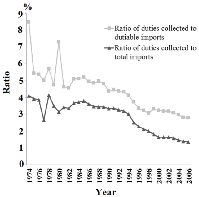
Source: Author’s computationfrom the data at The Center for International Data at UC Davis.
Figure 1 US average tariff

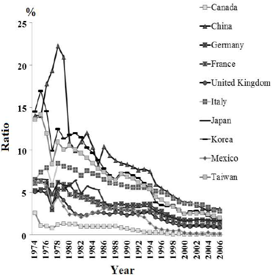
Source: Author’s computation from the data at CID at UC Davis.
Figure 3 US average tariff, 1974 to 2006, Ratio of duties collected to total imports
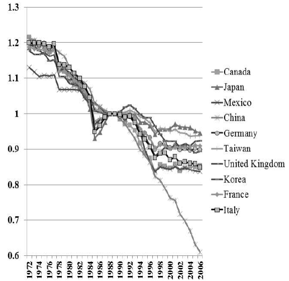
Figure 4 The evolution of the zero index in US imports from the 20 largest import partners plus Colombia and Chile: 1972-2006.


