


 text new page (beta)
 English (pdf)
 Article in xml format
 Article references
 Send this article by e-mail
 Cited by SciELO
  Similars in
SciELO
Similars in
SciELO 
 Permalink
Introduction
The study of time series classification has gained a great deal of interest due to the large amounts of information generated from the study of various phenomena that evolve in time. This dynamic behavior is observed in the biomedical areas such as disease studies, drug efficacy assessments, treatment analyses, signal processing, and image analysis, etc. where the importance of finding patterns that can help us to segment behaviors arises.
The complexity in time series classification stems from the inadequacy of traditional similarity metrics, which fail to account for the temporal aspect inherent in such data. These datasets frequently exhibit temporal relationships, shifts over time, and variations in magnitude, posing challenges for classification methods reliant on linear comparisons. Certain conventional approaches opt for an initial feature extraction phase to derive pertinent information from the data. However, given these limitations, there's a pressing need to explore alternative representations that remain invariant to shifts, preserve magnitudes, and retain temporal dependencies.
In [1], various techniques for time series classification across different domain representations are explored. These include methods based on dictionary representation, which involves counting the frequency of specific patterns within the data. Another approach involves extracting distinctive shapes, termed as shapelets, present within each class, enabling effective differentiation between groups. Additionally, one analysis strategy involves converting signals into images, leveraging our current computational capabilities to develop more sophisticated models, often relying on neural networks [2] [3] [4] [5] [6] [7].
This article's contribution lies in its exploration of three distinct methods for representing time series data, specifically applied to biomedical signals. These methods unveil various temporal relationships within the information, potentially enhancing classification performance. The study also delves into analyzing which representation proves most effective for each dataset and classifier, thereby shedding light on the optimal approach for different data contexts and classification algorithms.
In this paper, we aim to review three cutting-edge time series transformation methods, each tested with diverse hyperparameter configurations. These methods will be applied across five distinct biomedical datasets, each possessing unique properties. The objective is to thoroughly evaluate their efficacy in handling classification tasks within these varied biomedical contexts.
Materials and methods
Datasets
The article focuses on five datasets obtained from the UCR Time Series Classification Archive [8], which are widely acknowledged and frequently employed in state-of-the-art methodologies:
'SemgHandGenderCh2' (SHGC2): Captures surface electromyography signal power spectrum data depicting muscle electric activity during six hand grasp movements by five healthy subjects. These movements are categorized into two classes: Class 1 representing Female and Class 2 representing Male.
'PhalangesOutlinesCorrect' (POC): Centers on hand and bone outline detection, categorizing the output label as either a correct or incorrect image outline.
'CinCECGTorso' (CCECGT): Features data derived from ECG chlorine concentration readings across multiple torso-surface sites from four distinct individuals, each individual representing a single class.
'ECG5000': Revolves around ECG heartbeat recordings from a patient with severe congestive heart failure, with class values determined via automated annotation.
'UWaveGestureLibraryAll' (UWGLA): Comprises a collection of eight simple gestures generated from accelerometers.
Further details and characteristics of these datasets are available in Table 1. Notably, these datasets share the common characteristic of being univariate time series data, characterized by ndim = 1.
Table 1 UCR Datasets [8].
| Datasets | ||||
|---|---|---|---|---|
| Type | Name | Size | Class | Length |
| HAR | SemgHandGenderCh2 | 900 | 2 | 1500 |
| Image | PhalangesOutlinesCorrect | 2658 | 2 | 80 |
| ECG | CinCECGTorso | 1420 | 4 | 1639 |
| ECG | ECG5000 | 5000 | 5 | 140 |
| HAR | UWaveGestureLibraryAll | 9236 | 8 | 945 |
It's interesting to note that these datasets encompass three distinct types of data sources:
Human Activity Recognition (HAR): This category involves datasets like 'SemgHandGenderCh2' (SHGC2) and 'UWaveGestureLibraryAll' (UWGLA), which capture human movements and gestures, often derived from sensors or accelerometers.
Image Contours (Image): 'PhalangesOutlinesCorrect' (POC) falls under this category, focusing on the detection and assessment of image outlines, specifically related to hand and bone outlines.
Electrocardiogram Signals (ECG): Datasets such as 'CinCECGTorso' (CCECGT) and 'ECG5000' involve electrocardiogram data, primarily concerning the recording and analysis of heart-related signals, including chlorine concentration readings and heartbeat patterns.
Transformation methods
RandOm Convolutional KErnel Transform (ROCKET)
Convolutional kernels can be thought of as a matrix of values used to modify the input data by a dot product. These kernels contain certain basic parameters such as length, weights, bias, dilation, and padding. The kernels have the same 1-dimensional vector structure as the input data but are smaller in size. In the case of time series, the kernels are weighted vectors with a bias added to the result of the convolution between the input data and the kernel weights.
These kernels operate as filters, enabling the extraction of diverse shapes and patterns embedded within time series data. Through kernel dilation, these filters can extract patterns across various scales, reflecting different frequency characteristics. By leveraging a combination of multiple kernels, the system can extract complex patterns. While the weights of convolutional neural network kernels are typically learned, random convolutional kernels have demonstrated striking effectiveness.
ROCKET capitalizes on the concept of employing random convolutional kernels as a feature transformation for input in other classifiers. This transformation method offers a low computational cost owing to the random initialization of kernels instead of learned weights. As it involves a single layer, numerous kernels can be generated without significantly escalating the computational demand.
ROCKET employs a mechanism akin to max pooling by extracting maximum values from each feature map. However, it introduces a novel feature: the proportion of positive values. This addition enables ROCKET to discern the prevalence of a distinct pattern within the time series [9]. The process of this method is visually illustrated in Figure 1.

Gramian Angular Field
The Gramian Angular Field (GAF) is based on the dot product operation between two vectors, which shows the similarity that exists between them. If we have two vectors u and v with a norm of 1, we get Equation 1.
When working with unit vectors, the dot product is characterized only by the angle θ between u and v, since the magnitude of a unit vector is 1, which is why the result falls in the range [-1,1].
Considering the data as unit vectors, the Gramian matrix depicted in Equation 2 is formulated to capture linear dependencies within a vector set. This matrix serves to retain temporal dependencies, embedding the temporal dimension within the geometry of the matrix [10].
Given a time series X=x1, x2, … ,xn of n real observations, X is rescaled so that all values remain in the interval [-1,1] to preserve the unit vector property.
Once the information is scaled, the polar transformation is obtained. In this case, two values are considered:
From these values, the angle will be obtained, and this operation is described in Equation 3.
Some advantages of this coding are that it is a composition of bijective functions and that the temporal dependence is preserved based on the variable r_i. With these new angles, the dot product operation is adapted using Equation 4 so that it can be treated as a Gram matrix.
By implementing Equation 4 in G, the following Gramian matrix is obtained.
where cos(θ1+θ2) is given by Equation 6 in cartesian system.
This transformation generates a density map, portraying values through a color spectrum with intensities spanning from -1 to 1. Figure 2 illustrates a visual depiction of the encoded magnitudes.
Figure 2 Grammian angular field encoding sizes. a) 16X16 image. b) 24X24 image. c) 32X32 image. d) 48X48 image. e) 64x64 image.
Figure 3 showcases the distinct stages of this method, delineating the process involved in achieving the intended image representation.

Markov transition fields
Markov Transition Fields (MTF) offer an alternative method of transforming a time series into an image, employing a probabilistic framework rooted in Markov chains. This approach provides a distinctive perspective on representing time series data as visual elements.
Given a time series X=x1,x2,…,xn, its Q quantile bins are determined and each value x_i is assigned to its corresponding bin qj (j∈[1,Q]). From these bins, a weighted adjacency matrix W of size Q × Q is constructed, counting the transitions between bins in the form of a Markov chain along the time axis [10].
The calculation of wij is based on the frequency of occurrence where a point in quantile qj is succeeded by a point in quantile qi. After deriving this transition matrix, it undergoes normalization process to yield the matrix M. In this transition matrix, Mij represents the probability of transitioning from qi to qj. Leveraging these probabilities, we encode the time series into an N × N matrix, where N corresponds to the length of the original signal.
The color representation of the original signal is depicted through intensities ranging from [0, 1], delineated by the probability distribution. This image illustrates the likelihood of a point transitioning to other points (states) within the time series. Figure 4 showcases the visual encoding derived from this probability distribution.

For a comprehensive view of the method's process, please refer to Figure 5, which details the sequential steps involved in this encoding procedure.

All three of these transform representations are shown in Figure 6 for the same set of time series.

System and software specifications
This methodology was performed in a 11th Gen Intel® Core ™ i7-11800H processor with a NVidia GeForce RTX 3060 mobile GPU and 16 gb of DDR4 Sodimm.
The transformation methods were implemented using Pyts [11], and the classifiers were selected using the Scikit learn and tensorflow-keras packages [12] [13].
Pre-processing
Given the common occurrence of artifacts like noise and baseline offsets in biomedical signal data, a preliminary filtering stage was applied to enhance signal quality. To achieve this, a Savitzky-Golay filter was employed across all five datasets. This filter, widely used in biomedical signal processing [14], utilized a window size equivalent to 10 % of the signal length with a polyorder of 2. Notably, this filter retains essential characteristics of the initial distribution, including relative maximums, minimums, and peak widths, resulting in smoother signal behavior.
Additionally, Z normalization was performed to rectify baseline offsets, ensuring a consistent reference across all signal sets. This standardization establishes a zero mean and unit variance across the dataset, a technique known to often enhance model performance.
Once the whole dataset was ready, the training and testing subsets were created. The training set was defined as 70 % of the dataset size, the remaining 30 % was used for testing the classification models. 20 % of the training set was used as validation.
For comparison purpose, all three methods allow to define the output dimensions. On the image-based transformations it is defined by an N × N image where N ∈ {16,24,32,40,48\}. In ROCKET the response vector obtained is given by the number of kernels M generated times 2, the number of features extracted in every kernel, this equals to a 2M vector where M ∈ {625,1250,2500,5000,10000}.
Rocket
Other set of parameters that were random selected along all the kernels were, weights, bias, dilation, padding, the implementation can be seen in [9].
Gramian Angular Fields (GAF)
In GAF other variation parameters is the mode, in this case we have summation and difference mode.
Markov Transition fields (MTF)
For MTF the remaining variable parameter was the number of bins, this number gives us the number of states or resolution the data values can transition to. The number of bins was given by nBins where nBins ∈{8,16,32,64}.
All three transformations-ROCKET, GAF, and MTF- were applied across the five datasets, encompassing various combinations of parameters. These transformed datasets were utilized as inputs for the subsequent classification methods.
Classification methods
The classification stage aimed solely at evaluating transformation performance. The five datasets, transformed using distinct configurations, served as inputs for fixed classifiers to determine the input format that optimizes classification performance. No hyperparameter tuning was conducted on the neural network in this phase.
For the ROCKET-transformed data, a Ridge regressor classifier was utilized. This classifier incorporates a regularization parameter α within the loss function to prevent overfitting. Various values of α, selected from α ∈ {0.001, 0.01, 1, 10, 100, 1000}, were tested to identify the best-fitting parameter that avoids overfitting the model. Classifier selection was guided by references [9] [10].
In the case of image-based transformations, a convolutional neural network (CNN) with fixed parameters was employed. Categorical encoding was applied to the labels to optimize network functionality. The CNN architecture included the following modules:
input layer (image size)
convolutional layer (6 neurons, 8x8 size kernels)
max pool layer (3x3 pool size, padding=same)
convolutional layer (6 neurons, 3x3 size kernels)
max pool layer (3x3 pool size, padding=same)
flattening layer
dropout(0.5)
dense layer (categorical enconding = # labels, softmax)
The CNN utilized mean square error as the loss function, employed the adam optimizer, updated batch size weights of 50, and ran for 25 epochs. Figure 7 illustrates the various stages involved in evaluating the enhancement of time series transformations for classification.

Evaluation metrics
In the evaluation process, both mean square error (MSE) and accuracy were utilized to assess the performance of various input configurations and different parameter settings within the classifier. These metrics were computed on both the training and validation sets. To identify the most effective input configuration, the validation set's lowest MSE was considered.
For assessing test performance, metrics including accuracy, precision, recall, and f1-score were obtained. These measurements offer a comprehensive understanding of the model's predictive capabilities and effectiveness in correctly classifying instances.
Results and discussion
The preprocessing stage involved a stratification split to ensure an equal representation of class examples within the training and test sets. However, only the CinCECGTorso and UWaveGestureLibraryAll datasets exhibited an equal number of examples in each class.
Figure 8 demonstrates that ROCKET coupled with ridge regression exhibited notable performance, particularly with datasets where all classification test accuracies surpassed 0.8. One significant advantage observed in employing this method was its low memory resource consumption, as it did not require batch execution. Additionally, it was noted that the regularization parameter tended to perform better when α ≥ 1. However, the ECG5000 dataset showed poor precision, potentially due to class imbalance issues. It's important to note that the computing time for this method increased with a higher number of kernels, although the fitting process to the classifier was relatively swift once the data was transformed.
Figure 8 ROCKET transformation performance on the five datasets, number below each dataset correspond to (#kernels, α).
GAF, similar to ROCKET, showed promising performance on this type of data. However, certain limitations were observed, particularly with respect to memory consumption. Unlike ROCKET, the GAF transformation required batch processing for datasets larger than 1000 samples. Despite this limitation, the transformation process itself was rapid, as were the training times for the classifier.
Regarding the mode selection in GAF, it was noted that the difference mode yielded better results. Additionally, the optimal image size seemed to be 48. A detailed overview of performance results can be seen in Figure 9.
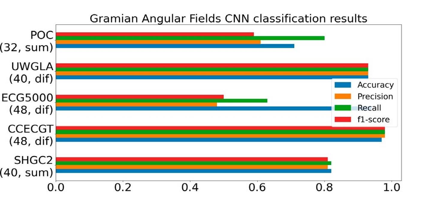
Figure 9 Gramian angular field transformation performance on the five datasets, number below each dataset correspond to (image size, transformation mode).
Finally, we conducted the MTF classification, yet this transformation didn't yield superior results compared to the preceding two methods. As illustrated in Figure 10, specifically in the precision column of ECG5000, MTF exhibited heightened sensitivity to quantile selection. Signals with low variability necessitated a smaller quantile size; larger quantile sizes led to certain bins containing only a few data points. Similar to the former method, MTF also required transformation into batches for signals exceeding a length of 1000 samples.
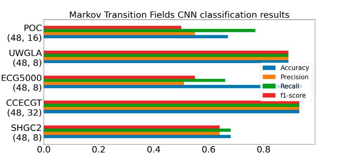
Figure 10 Markov transition field transformation performance on the five datasets, number below each dataset correspond to (image size, # bins).
The optimal outcomes were achieved with an image size of 48 and # bins set between 8 to 16.
In Figure 11 we summarize the F1 score on all datasets given by the optimal parameters for each transformation methods.

The computation time was systematically measured to analyze how signal size and the number of examples influence the time complexity of these methods. Observations revealed that while ROCKET consistently demonstrated better accuracy across all datasets, its computation time increased with a higher number of filters.
Conversely, GAF and MTF exhibited shorter transformation times, but they tended to consume more memory, scaling the information by N^2 where N represents the signal size. Additionally, MTF encountered challenges when discretizing time series with large bins and limited variability, preferring a smaller number of bins in such cases.
The time metrics were obtained by averaging the time taken for each transformation configuration across each dataset. These computation times are detailed in Table 2.
Table 2 Computation time measurements.
| Dataset mean computation time (seconds) | |||
|---|---|---|---|
| Name | ROCKET | GAF | MTF |
| SemgHandGenderCh2 | 30.7 | 1.8 | 5.7 |
| PhalangesOutlinesCorrect | 5.9 | 2.3 | 2.4 |
| CinCECGTorso | 51.8 | 2.0 | 9.7 |
| ECG5000 | 18.2 | 2.9 | 3.4 |
| UWaveGestureLibraryAll | 97.2 | 3.1 | 18.7 |
It's evident that these transformation methods serve as pivotal preprocessing steps, significantly enhancing the classification performance of these methods. The mean accuracy across all five datasets demonstrates strong performance: 0.936 for ROCKET, 0.874 for GAF, and 0.822 for MTF, all showcasing accuracies exceeding 0.8. This underscores their effectiveness in improving classification outcomes across diverse datasets.
For an overview of the key features and comparative analysis of each transformation method, please refer to Table 3.
Table 3 Methods observed characteristics.
| Comparison Table of methods | ||
|---|---|---|
| ROCKET | GAF | MTF |
| -Presents the highest accuracy of the three representations, with f1 scores over 0.6, even with unbalanced datasets. -The computation time increases linearly with the increase of number of kernels and the time series length. -It’s not image based, can be used with more traditional methods. -Due to the random initialization of the kernels, no hyperparameter tunning is required. |
-Presents the lowest computation time. -The accuracy obtained is lower than ROCKET, but comparable in some datasets. -Performance may increase with hyperparameter tunning on the NN or implementing other architectures. -Involves more hyperparameter for the transformation stage. -Memory consuming method. -Piecewise aggregate approximation is needed for high length data to avoid memory overflow. |
-Presents the lowest accuracy of all three methods. Struggles with unbalanced datasets. -Presents stability issues with high number of bins. -Has a fast computing time when transformation hyperparameters are well suited. - Involves more hyperparameter for the transformation stage. -Memory consuming method. -Piecewise aggregate approximation is needed for high length data to avoid memory overflow. |
Depending on the specific application and the tradeoffs you're willing to consider, you might opt for one method over another. Among all three, GAF demonstrated the most balanced performance concerning accuracy and utilization of time resources.
Additionally, these scrutinized time series transformation methods could prove beneficial in various machine learning tasks beyond classification, such as forecasting [15] [16] [17] [18] or clustering [19]. This can be explored in future work.
Conclusion
In this study, our primary focus was on transforming time series data to enhance classification performance. We introduced three distinct methods-Random Convolutional Kernel Transform, Gramian Angular Fields, and Markov Transition Fields-and rigorously tested their efficacy using five diverse biomedical datasets. The results illustrate that biomedical signals, when treated as time series data, can achieve classification performances akin to state-of-the-art methodologies [20] [21].
While our choice of classifiers was based on existing literature, it's crucial to note their adaptability to various other classifier types and architectures. For instance, in [10], a tiled Convolutional Neural Network was employed, with its last layer serving as input for a Support Vector Machine classifier. Different neural network architectures might yield comparable outcomes.
Notably, these imaging methods exhibit sensitivity to noise and generally perform optimally with signals less than 1000 samples in length due to memory constraints. However, they enable the extraction of diverse features from the data, significantly improving classification performance for temporal datasets.
For large-scale applications, the integration of deep learning computer vision approaches with attention mechanisms could leverage these representations, potentially offering promising outcomes in big data contexts.

