


 text new page (beta)
 English (pdf)
 Article in xml format
 Article references
 Send this article by e-mail
 Cited by SciELO
  Similars in
SciELO
Similars in
SciELO 
 Permalink
1. Introduction
This study is motivated by the importance of the sampled developing countries (Figure 1) in terms of economic growth, population, energy consumption, and pollutant emissions. According to World Bank data, in 2020 the 23 countries contributed with 33% to world GDP. The share of China and India was 18% and 3%, respectively. Economic growth and urbanization are interrelated to the pace of energy consumption and pollutant emissions (Santillán-Salgado et al., 2020). The rapid raise in urbanization is a propitious factor for economic activities, but it also creates many problems such as environmental degradation and higher energy demand (Wang et al., 2019). Regarding population, the studied countries had 60% of world population, with China and India roughly having the same number of inhabitants. In 2018, China consumed 21% of total world energy expressed in kg of oil equivalent, India 6%, and the other countries 13%. The preference for conventional fuels is behind the extraordinary release of CO2 emissions into the atmosphere (Liu et al., 2021; Mukhtarov et al., 2022). As seen in Figure 1, in 2014 China emitted 30% of CO2, India 7%, and the other countries 13%. Clearly, the studied developing economies are major participants in world economic growth, energy, and contamination.
Recently, empirical studies have introduced the variable of financial development in the energy-consumption literature (Sadorsky, 2010), although the nature of the relationship is complex (Belucio et al., 2019). In general, there are two hypotheses that explain the link between energy, growth, and carbon emissions (Sadorsky, 2011). The supply-side hypothesis states that financial intermediaries enhance economic growth by pooling resources from savers, and financing potentially profitable investment projects. Hence financial institutions could rise the level of productivity and the economic growth rate. Conversely, the demand-side hypothesis argues that economic growth raises the demand for financial services because they are intrinsically linked. Therefore, intermediaries foment higher energy consumption by consumers and businesses. However, as contended by Shahbaz et al. (2017), they can reduce energy consumption if they finance expensive renewable investment projects, for example. The inhibitory effect of finance on energy consumption works through the adoption of energy-saving and energy-efficient technologies, which would lead to lower atmospheric pollution (Khan et al., 2020)
The objective of this study is to question the link between energy consumption, CO2 emissions, financial development, and economic growth in developing countries. What is the Granger-causality among the mentioned variables? For this purpose, we use panel pairwise Granger causality (Dumitrescu and Hurlin, 2012) and GMM estimation of panel VAR-Granger causality with fixed effects (Abrigo and Love, 2016; Love and Zicchino, 2006). Neves et al. (2019) explain that the PVAR model of Love and Zichino (2006) is adequate because it overcomes the potential endogeneity among regressors; moreover, the GMM approach helps to control for country-specific effects and omitted variables (Khan et al., 2019). As for diagnostics, we apply Hausman tests, variance inflation factors (VIF), lag order selection, and cross-sectional dependence tests; and for model validation, we use impulse-response functions (IRF) and forecast-error variance decomposition (FEVD). The main conclusion is an interdependency between financial development, CO2 emissions, and gross domestic product (GDP); also, between CO2 emissions and primary energy consumption. Furthermore, we found unidirectional causality from electricity to CO2 and from financial development to energy consumption.
We contribute to the literature by ascertaining the causality of the nexus between electricity, primary energy, financial development (liquid liabilities and bank credit to private sector), carbon emissions, and economic growth in developing countries. Causality analysis and its direction is important for policymaking (Munir et al., 2020). For instance, if financial development Granger-causes energy consumption and CO2 emissions, then policymakers should implement appropriate policies to reduce carbon emissions without harming economic growth. However, if energy consumption causes financial development, this means that energy conservation policies will not affect the performance of financial institutions.
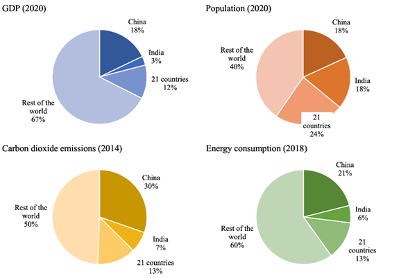
Source: own elaboration with data from the World Bank.
Figure 1 Share of GDP, population, CO2 emissions, and energy consumption in world totals
The rest of paper is organized as follows. Section 2 discusses the empirical evidence on the topic. The next section explains the data and the econometric approach. Section 4 describes the main results, while the discussion of Section 5 compares the results with related studies. Section 6 concludes.
2. Literature review
This section discusses the literature on linkage among energy consumption, carbon dioxide emissions, and economic growth. We emphasize the hypotheses underlying the causality among the variables of interest.
2.1 Energy, CO2 emissions and economic growth
Research on the causal linkage between energy and economic growth has been popular since the 1970s with the works by Griffin and Gregory (1976), Kraft and Kraft (1978), and Berndt and Wood (1979), as noted by Payne (2010). For example, Kraft and Kraft (1978), using the econometric method developed by Sims (1972), concluded that the gross national product leaded to energy consumption, thus introducing the issue of causality in the field. There are four known hypotheses of the Granger causality between energy and economic activity (Hajko et al., 2019; Rajaguru and Khan, 2021). The hypotheses are: (i) neutrality, (ii) growth (iii) conservation, and (iv) feedback.
In a major survey of papers published during 1974-2021, Mutumba et al. (2021) found that 10.5% of the results supported the neutrality hypothesis, 43.8% the growth hypothesis, 27.2% the conservation hypothesis, and 18.5% the feedback hypothesis. Given the growing number of papers published on the subject, it is unsurprising that no consensus has been reached. Mixed results have been attributed to different time periods, model specifications, empirical methods, and variables chosen (AlKhars et al., 2020; Jakovac, 2018; Mutumba et al., 2021; Payne, 2010). The first hypothesis states that energy consumption will not affect economic activity or vice versa. Also, energy policies will not induce changes in economic growth. Bulut and Muratoglu (2018) found for Turkey that renewable energy is not related to GDP growth nor there is causality between the two variables. Polat (2021) investigated the role of renewable and non-renewable energy consumption in GDP growth in developed and developing countries during 2002-2014. The author’s results support the neutrality hypothesis. For more evidence, see Akadiri et al. (2019), Banday and Aneja (2020), Wang et al. (2019), Charfeddine and Kahia (2019), Tugcu and Topcu (2018) and Shahbaz et al. (2020).
The growth hypothesis affirms that energy demand causes economic growth because it is an additional input to capital and labor in the production function. For example Gozgor et al. (2018) investigate the role of renewable and non-renewable energy consumption in the economic growth of 29 OECD countries during 1990-2013. Their long-run estimations with ARDL co-integration and quantile regressions confirm that a 1% increase in fossil energy consumption raises the rate of economic growth by 1.08%. Tang et al. (2016) examine the linkage between energy and growth in Vietnam over the 1971-2011 period using Johansen cointegration and the Toda-Yamamoto causality test. The authors confirm the hypothesis that energy consumption, along with foreign direct investment and capital stock, positively influence economic activity in Vietnam.
The conservation hypothesis states that energy policies aimed at diminishing energy consumption may not have a negative effect on economic activity. In fact, environmental activists and policymakers would expect this hypothesis to hold in the future to mitigate global warming (Hajko et al., 2019). For instance, Moftah and Dilek (2021) demonstrated that 16 Middle East and North Africa countries conformed to the conservation hypothesis. Moreover, Umurzakov et al. (2020) explore the energy-growth nexus in a panel data of 26 post-communist countries for the period from 1995 to 2014. By adding energy consumption to a traditional economic growth model with labor and capital, they proved empirically that economic growth drived energy demand.
Finally, the feedback hypothesis implies a mutual interconnection between economic growth and energy, as well as their joint behavior. In a study of 21 Latin American countries, Koengkan (2017) employed the PVAR methodology to analyze the relationship between primary energy consumption, economic growth, and urbanization. The results point out that energy consumption raises economic growth by 0.034% and that economic growth increases primary energy demand by 0.27%. Another example is Salazar-Núñez et al. (2020) that researches the causal links among primary energy consumption per capita, CO2 emissions per capita and GDP per capita. Using fully modified OLS and dynamic OLS, the authors deduced that for all the sampled countries there is a bidirectional causality between energy and growth in both the short- and long-runs.
In a study about the environmental effects of the North American Free Trade Agreement, Grossman and Krueger (1991) found that once per capita income is about $4,000 - $5,000 U.S. dollars, economic activity reduces environmental degradation. The finding is behind the so-called environmental Kuznetz curve (EKC) hypothesis (Apergis and Payne, 2020). This hypothesis states that at low levels of economic development, economic growth produces environmental degradation, which improves beyond certain limit of per capita income.
Regarding some evidence, Gessesse and He (2020) examine the interplay among carbon dioxide emissions, energy consumption, and economic growth in China. For the period 1971-2015, they concluded that economic activity accelerated energy consumption, and that carbon emissions leaded to economic growth (also, see Altinoz et al., 2020; Salazar-Núñez et al., 2020; Salazar-Núñez et al., 2021; and Oryani et al., 2021). On the other hand, Rahman (2020) studied the impact of electricity consumption, economic growth, and globalization on CO2 emissions in 10 top electricity consuming economies. Contrary to the previous work, in this study economic growth causes environmental degradation (Adebayo and Akinsola, 2021; for more on this topic, see Shaari et al., 2017; Li et al., 2021a; Li et al., 2021b).
2.2 Energy and financial development
Financial development matters for economic development (King and Levine, 1993a; King and Levine, 1993b). There exist two opposing views in the ample literature on finance and economic growth (Sadorsky, 2010). For the supply-side financial development, intermediaries influence economic activity through two channels (Ang, 2008; Levine, 1997). The capital accumulation channel refers to the intermediaries’ ability to pool resources and allocate savings to fund sectors and projects with potentially high investment rates. In turn, this process leads to higher capital accumulation and economic growth. The second channel, the total factor productivity channel, implies that financial institutions overcome informational asymmetries, thus improving allocation of resources, screening of investment projects, and adoption of more productive technologies (Greenwood and Jovanovic, 1990; Pagano, 1993; Venegas-Martínez et al., 2009).
Under the supply-side view, financial development Granger-causes energy consumption (Anton and Afloarei Nucu, 2020; Durusu-Ciftci et al., 2020; Gaies et al., 2019; Sadorsky, 2010). Intermediaries make access to funds easier for consumers to buy expensive items (i.e., refrigerators, washing machines, houses, cars, air conditioners, etc.) that tend to consume a lot of energy and influence the economy’s total demand for energy (direct effect). Firms also benefit from better financial development because they obtain financing for expanding or constructing offices and plants, buying more machines and equipment, or hiring new employees (business effect). Through the stock market, financial institutions enable firms to obtain less costly capital and promote the arrival of foreign direct investment, again pushing up the energy demand (wealth effect). Lastly, intermediaries help reduce economic risks and uncertainty which improve consumers and businesses’ trust in the economy.
Yue et al. (2019) explore the linkage between financial development and energy consumption in 21 transitional countries during 2006-2015. The panel smooth transition regressions (linear and non-linear effects) proved that banking intermediation (deposits and loans) had a positive effect on energy consumption. However, the stock market development caused a fall in Poland and China’s energy demand. Following Sadorsky (2010), Sadorsky (2011) shows that the banking sector (assets, deposits, and liabilities) and the stock market (turnover ratio) positively affected long-run economic growth. Durusu-Ciftci et al. (2020) examine the nexus among financial development, energy consumption, and economic growth in 21 countries. Overall, they found causality running from finance to energy conditional to economic development, e.g., in Mexico, Colombia, and Turkey. For further evidence, see Bass (2018), Mukhtarov et al. (2022), Danish and Ulucak (2021), and Shahbaz et al. (2021).
The demand-side view proposes that economic growth affects financial development (Robinson, 1952; Taivan and Nene, 2016). Raises in economic growth will increase the demand for financial services, given that they are intrinsically tied to the economy. Moreover, it is likely that “…energy demand should be relatively non-responsive to financial development” (Sadorsky, 2010, p. 2529). Considering this proposition, Ali et al. (2015) researches the finance-energy link in Nigeria with the ARDL bounds testing approach. Their long-run results show that financial development is non-responsive to energy demand. Moreover, Anton and Afloarei Nucu (2020) examine a sample of 28 European economies with data covering the period 1990-2015. The estimations indicate that banking development and the bond market have a positive effect on renewable energy consumption. However, they did not find any evidence for the capital market development.1
2.3 Research gap
As discussed in the literature reviewed, there is an unfinished debate on the nexus between energy, finance, and economic growth with the implied environmental degradation. Regarding economic growth, the evidence tends to marginally favor the growth hypothesis; however, in the financial development area, results are more mixed. On the other hand, for developing countries, only a few studies have jointly examined primary energy, electricity generation, CO2 emissions, financial development indicators, and economic growth (e.g., Jian et al., 2019; Shahbaz et al., 2013). We attempt to fill the gap in this study.
3. Data and econometric methodology
3.1 Data description
The annual data from 2001 to 2019 used in this study were obtained from the British Petroleum Statistical Review, the World Development Indicators and the Global Financial Development of the World Bank, the Bank for International Settlements, and the Economic Commission for Latin America and the Caribbean. Due to data availability, the sample consists of 23 developing countries: Algeria, Argentina, Bangladesh, Belarus, Brazil, Chile, China, Colombia, Ecuador, Egypt, the Philippines, India, Indonesia, Malaysia, Mexico, Morocco, Pakistan, Peru, Sri Lanka, South Africa, Thailand, Turkey, and Vietnam. The variables used in this study are described in Table 1.
Table 1 The description of variables
| Variables | Description and transformation | Symbols |
|---|---|---|
| Electricity generation | Terawatt-hours per capita, in natural logarithms and first difference | DELG |
| Carbon dioxide emissions | Million tonnes per capita, in logarithms and first difference | DCO2 |
| Primary energy consumption | Million tonnes oil equivalent per capita in logarithms and first difference | DPEC |
| Gross domestic product | Per capita, local constant unit, in logarithms and first difference | DGDPC |
| Bank credit to private sector | Per capita, local constant unit, in logarithms and first difference | DCSP |
| Liquid liabilities | Per capita, local constant unit, in logarithms and first difference | DLL |
| Inflation rate | Annual inflation rate in percentages | TINF |
Source: British Petroleum, the World Bank, Bank for International Settlements, and Economic Commission for Latin American and the Caribbean.
We decided to use panel data estimations because they have several advantages against alternative methods. First, data are more informative and there is less collinearity among variables, more degrees of freedom, and more efficiency (Anton and Afloarei Nucu, 2020; Baltagi, 2021). Second, multivariate analysis is more convenient since it avoids the problem of omitted variables, and therefore misleading conclusions (Durusu-Ciftci et al., 2020; Tang et al., 2016).
3.2 Model specification
After adjusting and extending the models proposed by Valencia-Herrera et al. (2020) and Alola et al. (2019), the model for this research is as follows:
For country
3.3 Econometric approach
The empirical approach of this study has four stages. In the first stage, we apply four diagnostic tests including the Hausman test, variance inflation factors (VIF), the lag order selection and cross-sectional dependence tests. For the second stage of pairwise analysis, we employ the panel Granger non-causality test of Dumitrescu and Hurlin (2012). The third stage of model estimation takes on estimating the PVAR-Granger causality Wald tests. Finally, the fourth stage of validity uses impulse-response functions (IRF), the eigenvalue stability condition, and the forecast-error variance decomposition.
To test for the existence of cross-dependence among panel units, we adopt the
tests of Pesaran et al. (2004) scale LM,
Breusch and Pagan (1980) LM, and Baltagi
et al. (2012) bias-corrected scaled LM.
In general, the tests compute the correlation coefficients among the variables
of unit
where
Next, we proceed with the bivariate analysis based on the recent panel Granger causality test proposed by Dumitrescu and Hurlin (2012). The test calculates individual Wald statistics of Granger non-causality that is averaged across panel units. Following Dumitrescu and Hurlin (2012) and Ozcan et al. (2020), the test can be computed from the following equation:
where
and the alternative hypothesis as:
In sum, we apply the pairwise analysis with the method proposed by Dumitrescu and
Hurlin (2012), but also with bootstrapped
Love and Zicchino (2006) used a panel-data VAR method that merges the traditional VAR model (all variables are assumed to be endogenous) with the panel approach (unobserved individual heterogeneity is assumed). The first-order vector autoregressive specification is written as:
In Equation (6),
4. Results
Table 2 shows the descriptive statistics of GDP per capita in local constant units (GDPC), electricity generation (ELG), carbon dioxide emissions (CO2), primary energy consumption (PEC), bank credit to private sector (CSP), liquid liabilities (LL), and the inflation rate (INF). The minimum values of ELG and PEC are 0.124 and 0.092 and their maximum values are 5.368 and 3.281, respectively. Given those values, we observe that ELG exhibits more dispersion than PEC (a standard deviation of 1.352 versus 0.782). However, in terms of environmental degradation, CO2 displays even more dispersion at 2.210 standard deviation. Regarding the financial development variables, that is, bank credit and liquid liabilities, their minimum value are 5.801 and 14.609, respectively, and their maximum values are 164.664 and 207.674, respectively. However, their standard deviations are roughly similar with 1.028 and 1.208 each. Moreover, inflation rates evince substantial dispersion (7.487 standard deviation). Therefore, in developing countries we observe marked disparities in environmental degradation than in energy consumption and financial development, as well as large macroeconomic instability.
Table 2 Descriptive statistics
| Statistics | GDPC | ELG | CO2 | PEC | CSP | LL | TINF |
|---|---|---|---|---|---|---|---|
| Min. | 2975.0 | 0.124 | 0.184 | 0.092 | 5.801 | 14.609 | -1.710 |
| Max. | 40459014.2 | 5.368 | 9.561 | 3.281 | 164.664 | 207.674 | 168.620 |
| Mean | 3297696.4 | 1.935 | 2.922 | 1.146 | 54.730 | 68.004 | 7.266 |
| Median | 51021.8 | 1.573 | 2.114 | 0.922 | 37.649 | 58.035 | 4.532 |
| Standard dev. | 8154779.0 | 1.352 | 2.210 | 0.782 | 41.100 | 38.052 | 11.988 |
| Skewness | 2.7 | 0.769 | 1.112 | 0.711 | 1.028 | 1.208 | 7.487 |
| Observations | 460 | 460 | 460 | 460 | 460 | 460 | 460 |
Source: Own elaboration using Stata v. 15.
The variance inflation factors, the cross-sectional dependence tests, and the Hausman tests are shown in Table 3. The VIF coefficients range from 1.5 to 2.250 and therefore those levels discard the presence of multicollinearity in the data. The Pesaran CD, the Breusch-Pagan LM, and biased-corrected scaled LM tests strongly indicate the presence of cross-sectional dependent in panel units.2 The estimation of the PVAR requires that in at least one of the equations the Hausman test be fixed effects (Neves et al., 2019), as specified in Equation (6). Neves et al. (2019) explain that the introduction of fixed effects causes correlation problems between the explanatory regressors. Nonetheless, the Hermelet procedure and the GMM’s system estimations, as argued by Arellano and Bover (1995), allow for the elimination of those problems. As seen in Table 3, in the equations for DELG and DCSP the Hausman tests are fixed effects.
Table 4 contains the results of the lag order
selection and the Hansen-J
Table 3 VIF, Hausman, and cross-sectional dependence tests
| Independent variables | Dependent variables | |||||||||||||
|---|---|---|---|---|---|---|---|---|---|---|---|---|---|---|
| DGDPC | DELG | DCO2 | DPEC | DCSP | DLLY | TINF | ||||||||
| DGDPC | -- | 1.620 | 1.830 | 1.800 | 1.650 | 1.830 | 1.820 | |||||||
| DELG | 1.470 | -- | 1.670 | 1.600 | 1.660 | 1.660 | 1.610 | |||||||
| DCO2 | 3.410 | 3.420 | -- | 1.400 | 3.410 | 3.420 | 3.420 | |||||||
| DPEC | 3.630 | 3.530 | 1.510 | -- | 3.690 | 3.680 | 3.690 | |||||||
| DCSP | 1.500 | 1.670 | 1.670 | 1.670 | -- | 1.390 | 1.600 | |||||||
| DLL | 1.370 | 1.370 | 1.380 | 1.380 | 1.150 | -- | 1.380 | |||||||
| TINF | 1.120 | 1.100 | 1.130 | 1.130 | 1.080 | 1.130 | -- | |||||||
| Cross-sectional dependence tests | ||||||||||||||
| Pesaran CD | 21.093 | *** | 10.828 | *** | 6.021 | *** | 6.797 | *** | 5.887 | *** | 8.073 | *** | 8.043 | *** |
| Breusch-Pagan LM | 852.252 | *** | 358.629 | *** | 340.845 | *** | 355.281 | *** | 477.761 | *** | 459.238 | *** | 586.360 | *** |
| Biased-corrected scaled LM | 26.011 | *** | 4.501 | *** | 3.266 | *** | 3.908 | *** | 9.353 | *** | 8.529 | *** | 14.181 | *** |
| Hausman test | 2.420 | 40.280 | *** | 2.280 | 5.660 | 17.550 | *** | 8.170 | 2.700 | |||||
Note: *** indicate significance at the 1% level.
Source: Own elaboration using Stata v. 15.
Table 4 Lag order criteria
| Lag | CD | J | J-P value | MBIC | MAIC | MQIC |
|---|---|---|---|---|---|---|
| 1 | 0.7375 | 144.1527 | 0.5510 | -704.7063 | -149.8473 | -371.3647 |
| 2 | 0.9706 | 90.5009 | 0.6922 | -475.4052 | -105.4991 | -253.1774 |
| 3 | 0.9767 | 52.6146 | 0.3359 | -230.3384 | -45.3854 | -119.2245 |
| 4 | 0.9511 | -- | -- | -- | -- | -- |
| Hansen-J test 𝜒2 | 90.501 |
Source: Own elaboration using Stata v. 15.
Regarding the pairwise analysis, the results from the panel Granger non-causality
test based on Dumitrescu and Hurlin (2012)
are in Table 5. The simple bivariate
relationships exhibit a feedback nexus between GDP and liquid liabilities. There is
unidirectional causality running from bank credit to GDP, liquid liabilities, and
primary energy consumption. On the other hand, liquid liabilities Granger-cause
primary energy and pollutants. In addition, carbon emissions Granger-cause primary
energy consumption, and DELG Granger-causes liquid liabilities but at the 10%
significance level. Overall, the bivariate analysis with bootstrapped
The bivariate analysis of financial deepening, energy, CO2 emissions, and
economic growth exclude joint interactions among the variables. Because of this
reason and based on Abrigo and Love (2016), we
proceed with the estimation of the Granger causality Wald tests (Table 6) where some new relationships emerged.
The null hypothesis is the nonexistence of causality between the tested variables;
therefore, the rejection of the null hypothesis implies that there is
Granger-causality between the variables. The results demonstrate several causalities
that reject the null hypothesis (we exclude inflation rates): DGDPC causes DLL; DELG
causes DCO2; DCO2 causes DPEC and DLL; DPEC causes DCO2; DCSP causes DGDPC, DCO2,
and DPEC; and DLL causes DGDPC, DCO2, and DPEC. To make the previous finding
clearer, Figure 2 displays the summary of
PVAR-Granger causalities. We grouped the banking variables into one variable,
i.e., financial development. According to the evidence for
developing countries, there exists bidirectional causality between financial
development and carbon dioxide emissions, between financial development and economic
growth, and between primary energy consumption and pollutant emissions. Moreover,
financial development affects primary energy consumption and electricity generation
Granger-causes carbon emissions. Then, to verify the stability condition of the
estimated model, we applied the eigenvalue stability condition (Table 7). The condition determines that there
is normality and stability, given that all eigenvalues are within the unity circle
and the imaginary and real values are within the range
Table 5 Dumitrescu and Hurlin (2012) Granger non-causality tests
| DGDPC | DELG | DCO2 | DPEC | DCSP | DLL | TINF | ||||||||
|---|---|---|---|---|---|---|---|---|---|---|---|---|---|---|
| Z bar | Z bar | Z bar | Z bar | Z bar | Z bar | Z bar | ||||||||
| a) Bivariate relationships | ||||||||||||||
| DGDPC | -- | -0.9634 | 0.0908 | -0.4801 | 1.9955 | ** | 2.8783 | *** | 4.1768 | *** | ||||
| DELG | -1.0167 | -- | 0.9832 | 1.5898 | -0.4216 | 0.2308 | 2.5395 | ** | ||||||
| DCO2 | 0.9072 | -0.0631 | -- | 1.3491 | 1.4249 | 2.8588 | *** | 2.5875 | ||||||
| DPEC | 1.0663 | -1.3509 | 2.3062 | ** | -- | 2.4476 | ** | 3.8198 | *** | 3.0973 | *** | |||
| DCSP | -0.2047 | -0.7498 | 1.4088 | 0.1476 | -- | 1.2890 | 7.6997 | *** | ||||||
| DLL | 3.0956 | *** | 1.9207 | -0.0194 | 0.9544 | 3.8192 | *** | -- | 3.8747 | *** | ||||
| TINF | 0.8347 | 1.8742 | * | 1.1543 | 0.602 | 3.1360 | *** | 6.9557 | *** | -- | ||||
| b) Bootstrapped p-values (300 repetitions) | ||||||||||||||
| DGDPC | -- | -0.9634 | 0.0908 | -0.4801 | 1.9955 | * | 2.8783 | ** | 4.1768 | ** | ||||
| DELG | -1.0167 | -- | 0.9832 | 1.5898 | * | -0.4216 | 0.2308 | 2.5395 | ** | |||||
| DCO2 | 0.9072 | -0.0631 | -- | 1.3491 | 1.4249 | 2.8588 | *** | 2.5875 | ** | |||||
| DPEC | 1.0663 | -1.3509 | 2.3062 | ** | -- | 2.4476 | ** | 3.8198 | *** | 3.0973 | ** | |||
| DCSP | -0.2047 | -0.7498 | 1.4088 | * | 0.1476 | -- | 1.2890 | 7.6997 | *** | |||||
| DLL | 3.0956 | ** | 1.9207 | ** | -0.0194 | 0.9544 | 3.8192 | -- | 3.8747 | ** | ||||
| TINF | 0.8347 | 1.8742 | ** | 1.1543 | 0.6020 | 3.1360 | ** | 6.9557 | *** | -- | ||||
Note: ***, **, and * indicate significance at the 1, 5 and 10% levels, respectively.
Source: Own elaboration using Stata v. 15.
Table 6 PVAR-Granger causality Wald test results
| Equation | Excluded | |||||||||||||
|---|---|---|---|---|---|---|---|---|---|---|---|---|---|---|
| DGDPC | DELG | DCO2 | DPEC | DCSP | DLL | TINF | ||||||||
| DGDPC | -- | 4.295 | 1.586 | 1.233 | 37.654 | *** | 38.627 | *** | 15.480 | *** | ||||
| DELG | 1.275 | -- | 0.438 | 0.786 | 0.854 | 0.149 | 2.574 | |||||||
| DCO2 | 871.000 | 12.208 | *** | -- | 34.465 | *** | 12.873 | *** | 13.004 | *** | 16.314 | *** | ||
| DPEC | 3.151 | 0.578 | 16.922 | *** | -- | 13.020 | *** | 6.932 | ** | 15.454 | *** | |||
| DCSP | 2.522 | 0.177 | 0.329 | 0.098 | -- | 2.187 | 0.112 | |||||||
| DLL | 7.023 | ** | 0.072 | 6.372 | ** | 4.461 | 2.681 | -- | 5.579 | * | ||||
| TINF | 7.383 | ** | 26.587 | *** | 2.654 | 3.304 | 29.159 | *** | 24.420 | *** | -- | |||
Note: ***, **, and * indicate significance at the 1, 5, and 10% levels, respectively.
Source: Own elaboration using Stata v. 15.
In addition, the impulse-response functions (IRF) exhibit that most variables recover after 5 years (Figure 3); that is, the time a variable takes to return to zero after being hit by a shock. The IRFs present the following responses of the variables:
An impulse to financial development (liquid liabilities and bank credit to the private sector) induces a positive response from carbon dioxide emissions. On the contrary, an impulse to CO2 emissions causes a negative response from financial development.
A shock to financial development produces an increase in GDP. Similarly, a shock to GDP triggers an increase in financial development.
An impulse to financial development causes an increase in primary energy consumption.
An impulse to primary energy consumption raises carbon dioxide emissions, and vice versa.
An impulse to electricity generation causes a positive response from CO2.
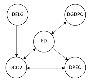
Source: Table 6.
Figure 2 Summary of PVAR-Granger causality relationships (excluding inflation rates)
Table 8 shows the outputs of the forecast-error variance decomposition (FEVD), which were computed with the Cholesky decomposition. The decomposition shows that in the first year DCO2, DCSP, and DLL explain most of their own variations (82.63%, 79.23%, and 61.71%, respectively). By the fifth year, DGDPC, DELG, and DPEC explain 92.81%, 62.36%, and 38.36% of their own variance, respectively. Moreover, by year 5,
The impulse of electricity generation and primary energy consumption on carbon dioxide emissions causes a raise of 8.8%.
GDP increases liquid liabilities by 39.16%, but together liquid liabilities and bank credit to private sector explain 2.29% of the forecast variance decomposition of GDP.
Pollutant emissions explain 2.39% of DLL and DCSP; on the contrary, the two variables explain 3.1% of the forecast variance behavior of DCO2.
Financial development explains 2.26% of the forecast error variance of primary energy consumption.
Overall, the IRFs and the FEVD imply that energy consumption (electricity and primary energy) are important sources of atmospheric contaminants in developing countries. In addition, there is bidirectional causality among financial development, GDP, and CO2 emissions. Such causality is consistent with the supply-side and demand-side hypotheses of finance, energy, and growth. For example, congruent with the demand-side finance hypothesis, economic growth promotes financial development. If this hypothesis is true, development of financial institutions increases energy demand and thereby carbon dioxide emissions. Either way, the performance of financial intermediaries has an influence on energy consumption and carbon dioxide emissions.
Table 7 Eigenvalue stability condition
| Real | Imaginary | Modulus | Roots of the companion matrix |
|---|---|---|---|
| 0.000 | 0.837 | 0.837 |

|
| 0.651 | 0.000 | 0.651 | |
| -0.351 | 0.404 | 0.535 | |
| -0.351 | -0.404 | 0.535 | |
| -0.455 | 0.000 | 0.455 | |
| 0.320 | -0.310 | 0.446 | |
| 0.320 | 0.310 | 0.446 | |
| -0.039 | 0.431 | 0.433 | |
| -0.039 | -0.431 | 0.433 | |
| -0.380 | 0.000 | 0.380 | |
| -0.133 | -0.297 | 0.326 | |
| -0.133 | 0.297 | 0.326 | |
| -0.276 | 0.000 | 0.276 | |
| 0.199 | 0.000 | 0.199 |
Source: Own elaboration.

Table 8 Forecast-error variance decomposition (FEVD)
| Response variable and forecast impulse variable horizon | Impulse variable | |||||||
|---|---|---|---|---|---|---|---|---|
| DGDPC | DELG | DCO2 | DPEC | DCSP | DLLY | TINF | ||
| DGDPC | 1 | 1 | 0 | 0 | 0 | 0 | 0 | 0 |
| 5 | 0.9281 | 0.0002 | 0.0047 | 0.0027 | 0.0107 | 0.0122 | 0.0414 | |
| 10 | 0.9238 | 0.0002 | 0.0044 | 0.0031 | 0.0095 | 0.0116 | 0.0474 | |
| DELG | 5 | 0.2243 | 0.6236 | 0.0565 | 0.0222 | 0.0136 | 0.0049 | 0.0548 |
| 10 | 0.2465 | 0.6038 | 0.0548 | 0.0217 | 0.0133 | 0.0050 | 0.0550 | |
| DCO2 | 1 | 0.0668 | 0.1070 | 0.8263 | 0 | 0 | 0 | 0 |
| 5 | 0.1135 | 0.0880 | 0.6966 | 0.0358 | 0.0192 | 0.0118 | 0.0352 | |
| 10 | 0.1338 | 0.0857 | 0.6782 | 0.0353 | 0.0189 | 0.0119 | 0.0361 | |
| DPEC | 1 | 0.0972 | 0.1186 | 0.4342 | 0.3501 | 0 | 0 | 0 |
| 5 | 0.1141 | 0.0893 | 0.3478 | 0.3836 | 0.0148 | 0.0078 | 0.0425 | |
| 10 | 0.1281 | 0.0875 | 0.3412 | 0.3773 | 0.0147 | 0.0079 | 0.0432 | |
| DCSP | 1 | 0.1946 | 0.0010 | 0.0011 | 0.0110 | 0.7923 | 0 | 0 |
| 5 | 0.4925 | 0.0024 | 0.0101 | 0.0067 | 0.4363 | 0.0079 | 0.0441 | |
| 10 | 0.5622 | 0.0020 | 0.0088 | 0.0061 | 0.3661 | 0.0092 | 0.0456 | |
| DLL | 1 | 0.1020 | 0.0029 | 0.0050 | 0.0076 | 0.2655 | 0.6171 | 0 |
| 5 | 0.3916 | 0.0026 | 0.0138 | 0.0059 | 0.1562 | 0.3440 | 0.0859 | |
| 10 | 0.4529 | 0.0023 | 0.0125 | 0.0057 | 0.1381 | 0.3045 | 0.0841 | |
| TINF | 1 | 0.0043 | 0.0010 | 0.0003 | 0.0595 | 0.1595 | 0.0113 | 0.7640 |
| 5 | 0.0168 | 0.0045 | 0.0074 | 0.1064 | 0.1264 | 0.0567 | 0.6820 | |
| 10 | 0.0168 | 0.0045 | 0.0074 | 0.1063 | 0.1266 | 0.0567 | 0.6816 | |
Source: Own elaboration.
5. Discussion of results and policy implications
Policymakers in developing countries would find useful the insights from this study about the interactions between financial development, energy consumption, electricity generation, CO2 emissions, and GDP. By using panel VAR Granger causality tests, our results show unidirectional causality from eletricity generation to carbon emissions and from financial development to primary energy consumption; also, bidirectional between finance and CO2, GDP and finance, and energy consumption and CO2. Moreover, the impulse-response functions in Figure 3 helps us to infer the sign of the causalities.
Firstly, regarding electricity generation and CO2 emissions, in the short run a one standard deviation shock to DELG increases pollutants in one year, although the effects decrease somewhat in the next years. The impact of electricity on CO2 is in line with some previous studies. In an analysis of Chile with ARDL, FMOLS, and DOLS estimations, Kirikkaleli et al. (2022) concluded that both GDP and electricity consumption raise consumption-based CO2 emissions. Naminse and Zhuang (2018) analyze the Chinese economy with dynamic OLS, Granger causality, and impulse-response functions for the period 1952-2012. The results indicate that electricity, coal, and oil-based consumption have a positive impact on air pollution Therefore, in developing countries policymakers could achieve short-run climate-change goals by using environmentally friendly technologies in the electricity sector.
Secondly, we observe a connection between the feedback link of financial development and GPD, and FD and CO2. The development of financial intermediaries pushes up economic growth, which provokes higher energy consumption and carbon dioxide emissions. On the contrary, as explained in the literature review section of this study, the opposite is true as inferred from the demand-side finance hypothesis. According to the estimated IRFs in this study, a shock to GDP increases financial development in the short run (year 1 for bank credit and year 2 for liquid liabilities), which vanishes by year 5. This is congruent with the evidence available for the cases of Saudi Arabia (Xu et al., 2018), BRICS countries (Rafique et al., 2020), the Gulf Cooperation countries (Baydoun and Aga, 2021), 25 Afrian countries (Khoshnevis Yazdi and Ghorchi Beygi, 2018), and European countries (Jamel and Maktouf, 2017; Manta et al., 2020).
On the other hand, we also found unidirectional causality from FD to primary energy consumption, which is in accordance with the previous interdependencies. There is abundant literature reporting evidence on such causality (Khan et al., 2019). It is worth mentioning that policymakers in less developed economies should implement policies to promote the deepening and efficiency of financial institutions to boost economic growth, while at the same remain vigilant of air-pollution levels.
According to our results, carbon dioxide emissions are responsible for primary energy consumption, whereas primary energy consumption affects air pollutants. An innovation to energy consumption reduces CO2 emissions by year 3; then, they increase until year 5. On the contrary, the response of energy consumption to a shock to air-pollutants is quite mixed and stabilizes after year 8. Some studies have found similar results. Gökmenoğlu and Taspinar (2016) use the case of Turkey to examine the nexus between carbon emissions, energy consumption, GDP, and foreign direct investment. Their Toda-Yamamoto causality tests show a feedback relationship between energy consumption and CO2. Another example is Shahbaz et al. (2013) who investigate the link between growth, energy consumption, financial development, trade openness, and CO2 emissions in Indonesia during the 1975-2011 period. Using ARDL and VECM Granger causalities, they confirm the hypothesis of a feedback nexus between energy consumption and air contaminants.
Finally, with the panel VAR estimations we did not obtain a direct relationship between economic growth, energy consumption and carbon emissions, which confirms the neutrality hypothesis. However, the other results from the analysis imply an indirect nexus between growth and energy. For example, by affecting financial development positively, economic growth is indirectly creating CO2 emissions because institutions would finance consumption and business activities (as discussed above about the causality from DFD to DPEC). Some of the studies that support this finding are Tuna and Tuna (2020) Gorus and Aydin (2019), and Dinç and Akdoğan (2019).
6. Conclusions
This study investigated the relationship between financial development (bank credit to private sector and liquid liabilities), energy consumption (electricity generation and primary), carbon dioxide emissions, and economic growth in a sample of 23 developing economies covering the period of 2001-2019. As a control variable, we included annual inflation rates. For this purpose, we applied pairwise analysis with the Granger non-causality test proposed by Dumitrescu and Hurlin (2012) and Abrigo and Love (2016). The second part of the bivariate analysis is based on bootstrapped p-values with 300 repetitions. To surpass the shortcomings of the pairwise analysis, we then proceeded to estimate a panel VAR-Granger causality. The panel VAR is later combined with impulse-response functions and forecast-error variance decompositions to have a better understanding of the directions of the causalities.
With pairwise analysis based on bootstrapped
These results are clearly important for policymakers in developing countries. The interplay between financial development, economic growth, and carbon dioxide emissions suggest that macroeconomic and energy policies should be carefully implemented to avoid unnecessary increases in atmospheric contamination. Regarding financial development, policymakers should implement polices aimed at improving the efficiency of institutions, while at the same time encouraging the adoption of greener technologies. Another tool to reduce CO2 emissions in the short run is through the electricity sector and primary energy, because our results underlined the positive causality between them and pollutants. Lastly, we did not find a direct relationship between GDP, energy, and carbon emissions, which supports the neutrality hypothesis. However, as we pointed out, economic growth influences indirectly energy consumption and carbon emissions.
One limitation of this study is the lack of enough data to apply further testing, i.e., cointegration tests. Based on cointegration tests, it would be important to understand the long-run behavior of the variables analyzed in this research. Another limitation is that it focuses solely on developing economies. Certainly, the introduction of developed economies into the analysis would enrich our understanding. Future research should consider the two limitations in the analysis to design and implement better climate-change policies.

