


 nueva página del texto (beta)
 Artículo en XML
 Referencias del artículo
 Enviar artículo por email
 Citado por SciELO
  Similares en
SciELO
Similares en
SciELO 
 Permalink
Introduction
In many kinds of statistical studies, including seismological ones, it is a common task to compare some observed probability distribution P={p j ; j=1,…,M} with some reference distribution Π={π j ; j=1,…,M}, and the difference between them is often measured by using the Kullback-Leibler divergence (K-L) κ:
(Kullback and Leibler, 1951; Eguchi and Copas, 2006). This measure is zero when P=Π, but it does not have a fixed upper limit; it can be infinite when one or more π j ’s are zero and the corresponding p j ’s are not (Lin, 1991; Shlens, 2007), but, for a reasonable reference distribution with no unbalanced zeros, how large can it be? It is necessary to have a reference value in order to assess the significance of any result other than zero.
In what follows, we will present a method for evaluating the confidence that can be had about two distributions being similar, based on a K-L measure, using a seismological example.
In assessing seismic hazard for a given region a common tool is to look for clustering or gaps in the times of occurrence of earthquakes above a given magnitude in the background seismicity, because those features may be precursors to a large earthquake. If the observed seismicity appears to show clusters or gaps, to assess their significance it is necessary to test whether they may be due to random concentrations in events occurring with uniform probability over time, i.e. to test the observations versus the null hypothesis.
One way to test the null hypothesis is to use the well known fact that if events are occurring randomly with uniform probability in time at a rate of λ events per unit time, then the number of events n occurring within intervals of a given length T are distributed according to the Poisson distribution:
(e.g. Mack, 1967; Dekking et al., 2005; Boxma and Yechiali, 2007), so we will compare the distribution of observed n’s with the Poisson distribution using the K-L divergence.
Significance of the K-L measure
Suppose that the times of occurrence of N e =160 earthquakes ocurred over a period N y =60 years have been observed, as shown in Figure 1 (top), which gives an occurrence rate λ=2.6̅6̅6̅6̅6̅ events/year, and , for the sake of simplicity, let us consider yearly intervals so T=1.0 yr in (2). Figure 1 (middle) shows the number of events per year, n, for each observed year, and (bottom) the corresponding histogram, as well as the expected number of events from the Poisson distribution.
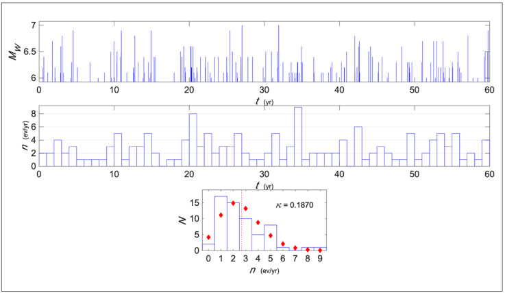
Figure 1 Times of occurrence 160 earthquakes with Gutenberg-Richter distributed magnitudes over a period of 60 years (top), number of earthquakes per year for each year (middle), and (bottom) histogram of numbers of earthquakes per year (blue line) and expected frequencies of earthquakes per year from the Poisson distribution.
The two distributions are not equal but, quantitatively, how different are they? We will measure their divergence using K-L. Observed probabilities are estimated from the histogram as
where N n is the observed number of incidences of n events/ year and n max is the maximum observed n. We will compare this observed probability distribution with the reference
as shown in Figure 2.
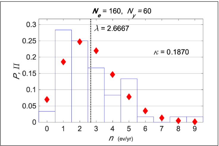
Figure 2 Observed distribution of n and corresponding values from the Poisson distribution (red diamonds) for λ=2.6̅6̅6̅6̅6̅ events/year indicated by the vertical dashed line. The K-L divergence between the two distributions is κ=0.1870.
To evaluate the K-L divergence between these two distributions, although the Poisson distribution is non-zero for an infinite number of terms, the summation in (1) is only done from 0 to n max , because P can be considered equal to zero for n>n max and terms with p n =0 do not contribute to the summation.
The K-L evaluation yields κ=0.1870, but, what does this number mean (apart from the distributions not being equal)? Here, it must be considered that, as is common for seismological studies, particularly those involving large magnitudes, the observed distribution comes from only one very short realization consisting of only N y =60 events.
Let us estimate how probable is the observed κ for samples of size N y of a Poisson process. We will do this through a Monte Carlo simulation (Yakowitz, 1977; Rubinstein and Kroese, 2016) of N r =100,000 realizations of synthetic samples of N y Poisson distributed numbers n; the divergence κ between the resulting distribution P and Π from (3) is evaluated for each realization.
The probability distribution f(κ) resulting from the simulation is shown in Figure 3 (top), the distribution has mean μ κ =0.1066 and standard deviation σ κ =0.0499, and it is clear that the probability that a 60 samples long random realization of a Poissonian process actually results in κ=0 is extremely small. Indeed, if the sampled process were indeed Poissonian, instead of κ=0, a value around κ=0.082 would be much more probable.
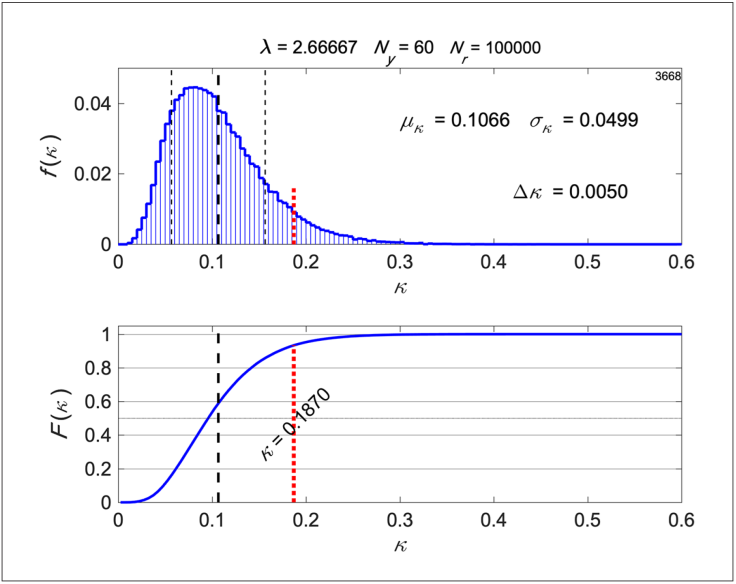
Figure 3 Distribution of κ values from the Monte Carlo simulation (top), ∆κ is the class width, the dashed thick vertical line indicates the mean μ κ of the N r =100,000 realizations, and the thin dashed vertical lines indicate plus/minus one standard deviation σ κ from the mean. Cumulative κ distribution (bottom), the dashed black line is μ κ , and the dotted red line indicates the observed κ=0.1870.
The cumulative F(κ) in Figure 3 (bottom) shows the observed κ=0.1870, and gives Pr(κ≥0.1870)=0.0664, so the possibility of the null hypothesis, that the observed seismicity occurred with uniform probability in time, can be rejected with 0.9336 confidence. This number constitutes a firm basis for the decision of whether to reject the null hypothesis or not; in this case the observed seismicity is, with high probability, not distributed uniformly in time, although the null hypothesis cannot be rejected at the widely used significance level of 0.05. It should be pointed out that this confidence estimation takes into account the sample length.
Other reference measures
We have presented a practical way for assessing the significance of a K-L measurement. Now, just for argument’s sake, let us consider two other reference measures.
First, consider the uniform distribution, which is a common reference because it has the highest entropy (Shannon, 1948), with probabilities
shown as circles in Figure 4 (left). The K-L divergence between the uniform and Poisson distributions for n max =9 is κ U =1.22055, much higher than the value for our example distribution and has a probability value of nearly zero.
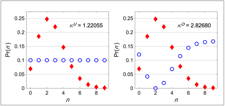
Figure 4 Poisson distribution for λ=2.6̅6̅6̅6̅6̅ events/year, and n max =9, indicated by red diamonds, and the uniform (left) and opposite (right) reference distributions.
The second reference distribution is the “opposite” distribution to Poisson:
where π max is the maximum value of the Poisson distribution. It is an inverted and normalized Poisson as shown by circles in Figure 4 (right). The K-L divergence for the opposite distribution is κ O =2.82680, and it is considerably higher than the observed κ and the reference κ U ; its divergence is not the highest possible between the Poisson distribution and another distribution of the same length, but it is the most different distribution in an intuitive way.
Of course, both reference values should be estimated for the same n range as that of the observed distribution (they increase with the length of the range), and may not be very useful because they have very large κ values with vanishingly small probabilities, but still they are better reference values than infinity.
Discussion
We presented a method of estimating significance levels associated with measures of the K-L divergence, and proposed two possible reference values. The Poisson distribution was used as an example, but the method is applicable to any other reference distribution.
The Monte Carlo evaluation of the significance of a κ value illustrates quite clearly the problem of having to work with small samples, which is unfortunately the case with many studies in statistical seismology, due to the relative shortness and heterogeneity of the seismic catalogs, particularly for studies dealing with large earthquakes. One of the advantages of the proposed method is that it takes into account variations caused from samples that are but small realizations of a stochastic process. In the example presented here we showed that a N y =60 long sample from a true Poissonian process has almost null probability of resulting in κ=0, because for that sample length the κ values are distributed with mean μ κ =0.1066 and standard deviation σ κ =0.0499, while samples of N y =120 have μ κ =0.0561 and σ κ =0.0255, and for N y =180 μ κ =0.0384 and σ κ =0.0171 (all for equal λ). Hence, κ values cannot be correctly interpreted without taking into account the sample length, something that our proposed method does implicitly.
The method proposed here can be a useful tool in studies of seismic hazard, where it is essential to distinguish, with a quantitative bas is, between an apparently anomalous distribution being observed and the null hypothesis.

