


 nueva página del texto (beta)
 Inglés (pdf)
 Artículo en XML
 Referencias del artículo
 Enviar artículo por email
 Citado por SciELO
  Similares en
SciELO
Similares en
SciELO 
 Permalink
Introduction
Because of its relatively better quality (compared to surface water) and its potential ubiquity, groundwater plays a very important role in water resources management policies. However, aquifers that provide groundwater are mostly characterized among others by the hydraulic conductivity (Arétouyap et al., 2015). Indeed, the modelling and the behaviour of the groundwater during the upcoming exploitation strongly depend on this parameter as it informs us about the recharge capacity of the aquifer (Asfahani, 2007).
Nowadays, because of the imprecision and the low efficiency of the traditional methods of pumping test, geo-electrical methods are increasingly used since the late 70s through the world to model and predict groundwater behavior during the upcoming exploitation (Kelly, 1977). Jones and Bufford (1951) and Croft (1971) established a sound relationship between permeability and formation factor. Similar relationships were established between resistivity and well productivity (Vincenz, 1968), transmissivity and transverse resistance (Ungemach et al., 1969), saturated thickness resistivities and hydraulic conductivities (Kelly,1977), aquifer transmissivity and transverse resistance (Mazác and Landa, 1979). Scarascia (1976) estimated the transmissivity through interpreting the electrical soundings in Italy. Asfahani (2007) applied the vertical electrical soundings technique to characterize the Neogene aquifer (Salamiyeh region in Syria) in terms of hydraulic conductivity, transmissivity, transverse resistance and thickness. Tahmasbi-Nejad (2009) and Anomohanran (2013) used also this resistivity method to study the water potential in areas of Behbahan-Azad (Iran) and Ukelegbe (Nigeria) respectively. Asfahani (2013 NO SE ENCUENTRA; 2016) used surficial vertical electrical sounding technique (VES) to compute the aquifer hydraulic conductivity. Those alternative approaches have been successfully applied for characterizing the transmissivity of the Quaternary and Paleogene aquifers in the semi-arid Khanasser valley region (Northern Syria), and for determining the hydrodynamic parameters of the Pan-African aquifer in the Adamawa-Cameroon region (Arétouyap et al., 2015).
More recently, Asfahani (2016) developed a new practical and easy approach for computing the hydraulic conductivity of aquifer by taking into consideration only the groundwater salinity. The main objectives of the present paper are therefore the following:
to check the efficiency and the effectiveness of the recent Asfahani (2016)'s method, by applying his approach in another region than Syria;
to use his method to locate and characterize local aquifers in terms of hydraulic conductivity and in order to re-compute the hydraulic parameters of the Pan-African aquifer in the Adamawa-Cameroon region;
to compare the results of hydraulic conductivity and the transmissivity obtained by Asfahani's approach with those obtained previously.
Previous geophysical research
In hydrological terms, 150 to 300 km wide, the Adamawa plateau is called "the water tower of the region" because it feeds three of the four major watersheds of the country. The most recent hydrogeophysical survey conducted in the region (Arétouyap et al., 2015) enabled to infer major hydrodynamic parameters of the local aquifers. It revealed that almost all of them are made of the fractured portion of the granitic bedrock located at a depth ranging between 7 and 84 m, the thickness between 1 and 101 m, the resistivity between 3 and 825 Ω.m, the hydraulic conductivity between 0.012 and 1.677 m/day, the transmissivity between 0.46 and 46.02 m2/day, and the product Κσ between 2.1×10⁻⁴ and 4.2×10⁻⁴. Those results were derived from an empirical relationship established by Arétouyap et al. (2015) between the aquifer resistance R and the product Κσ, in a region considered as a single uniform geological unit.
Geomorphology and hydrogeology of the Adamawa Plateau
This study is conducted in the Adamawa-Cameroon region, located in the heart of Central Africa between 6° - 8° north and 11° - 16° east (Figure 1). The study region extends over a length of about 410km from west to east between the Federal Republic of Nigeria and the Central African Republic, with an area of 6782 km2. The morphology of the region is of volcanic highlands, resulting from tectonic uplift and subsidence accompanied by intense magmatic emissions (Vincent, 1970; Tchameni et al., 2001). Although the average altitude is 1100 m, this region of a rugged terrain is limited at the North by a large cliff and an uneven escarpment of several hundred meters that dominates the area.
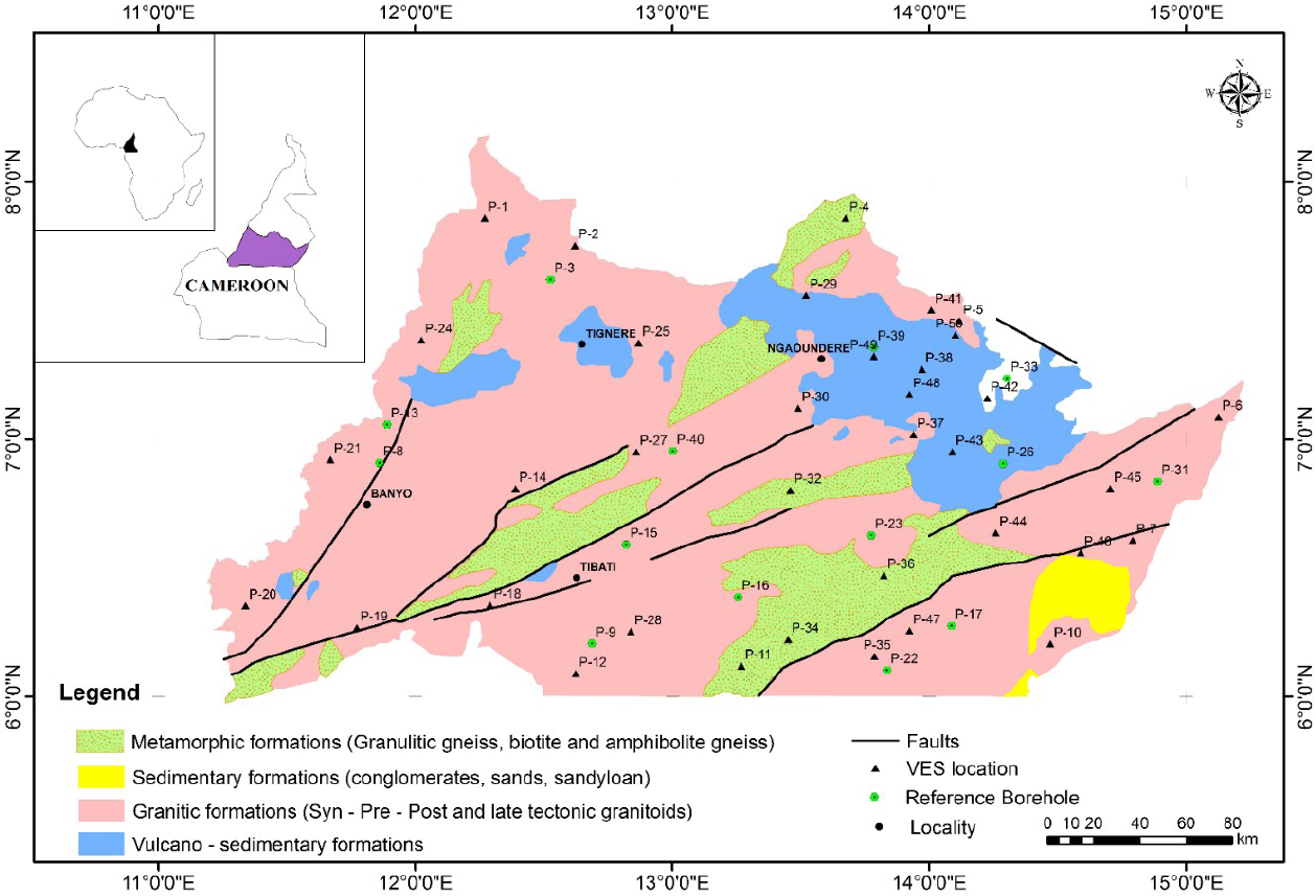
Figure 1 Geological map of the study area, with the locations of VES measurements (Maréchal, 1976) as amended.
The center of the plateau is marked by soft forms barely accented and swampy valleys, dotted with mountains or/and volcanic cones. At the East, there are massifs resulting from the former erosion and tectonic movements around the regions of Meiganga and Bagodo. In the West, the terrain is mountainous with hills. Volcanic inheritance covers the North, the East and the South areas. One notes the presence of an assembly line which occupies an important part of the region, reaching altitudes greater than 2240 m at Mount Tchabal-Mbabo. There are also plains and basins such as the Tikar plain in the Mayo-Banyo division. The southern part is characterized by a huge plateau that gradually drops until the penepla in Djerem (Toteu et al., 2000).
The geological history of the Adamawa-Cameroon region is marked by three major events (Toteu et al., 2000):
— A long period of continental erosion from Precambrian to Cretaceous;
— The onset of volcanism from Cretaceous to Quaternary;
— Recurrent basement tectonics that explain the horst and graben structure of the region.
An investigation of superficial formations in the region has highlighted the Pan-African granite-gneiss basement, represented by Ordovician granites, gneisses and Pan-African migmatites. The main geological units present inthe study region are basalts, trachytes and trachyphonolites based mostly on concordant ttcalco-alkaline granites and discordant alkaline granites (Toteu et al., 2000). The presence of metadiorites of Paleoproterozoic basement it is also observed (Toteu et al., 2001). According to the same authors, major fractures of the Pan-African bedrock fall into two main directions:
— The most common direction oriented N 30 °E, is that of the "volcanic line of Cameroon";
— The second directed N 70 °E, corresponds to the "line of Adamawa" or "Adamawa shear zone".
Geophysical surveys revealthat the bedrock of the study area is intensely faulted (Robain et al., 1996; Cornacchia and Dars, 1983; Dumont, 1986; Ngako et al., 2008; Njonfang et al., 2008; Toteu et al., 2004). Such tectonic activities augur potential existence of groundwater in the region. However, apart from Arétouyap et al. (2015) that considered the whole region as a single geological unit, there is no recent study to locate and characterize the local aquifers. This situation justifies the interest of the present paper.
Methodology
VES data recording and interpretation
A vertical electrical sounding (VES) with Schlumberger configurationis conducted in the region in order to locate and characterize the aquifers in the study region. With this technique, the electrical resistivity variations are expressed as a function of depth. Fifty vertical electrical soundings (VES) including 14 with available water samples have been conducted in the region using the Terrameter ABEMSAS-1000 with a spacing of current electrodes (AB) varying from 2 to 600 m.
In the present research, the curve matching technique is used to set structural parameters (Orellana and Mooney, 1966). Then, an inverse technique algorithm developed by Zohdy (1989) and Zohdy and Bisdorf (1989) fits both theoretical and field curves for each experimental. Dey and Morrison (1979) mentioned the possibility of considering and assuming the medium to be as a one-dimensional model (1D). The geological conditions in the study area were favorable and allowed us to assume and apply the 1D model. The 1D quantitative interpretation of the 50 VES has already enabled the identification of geoelectrical characteristics of the Pan-African deposits (Arétouyap et al., 2015).
Hydraulic conductivity estimation
This section is the main core of the survey. The hydraulic conductivity is estimated by using the approach proposed by Asfahani (2016), which consists of the seven steps reminded below.
Determination of the water resistivity ρ w
14 experimental VES measurements are carried out in the vicinity of available water samples (boreholes in function). Values of water conductivity (σW) from those 14 available water samples are measured, their water resistivity (ρ w) values are thereafter deduced by using equation 1.
Hence, the factor formation (F) used in Archie's law becomes a function of both σW and (ρ w).
Those 14VESs have been quantitatively interpretedusing curve matching method (as illustrated in Figure 2), where the resulting resistivity (ρ rock ) and thickness (h) values are shown in Table 1.

Table 1 Hydrological and geophysical parameters of 14 reference VES.
| VES | ρrock (Ω.m) | ρw (Ω.m) | h (m) | TR (Ω.m2) | MTR (Ω.m2) | F | K (m/day) | T (m2/day) |
|---|---|---|---|---|---|---|---|---|
| P-3 | 472.0 | 2.03 | 8.4 | 3964.8 | 5856.5 | 157.4 | 0.62 | 2.4 |
| P-8 | 134.0 | 3.21 | 43.0 | 5762.0 | 5382.5 | 44.7 | 0.09 | 12.4 |
| P-9 | 207.0 | 5.01 | 19.0 | 3933.0 | 2354.0 | 69.0 | 0.09 | 5.5 |
| P-13 | 177.0 | 1.68 | 48.0 | 8496.0 | 15164.2 | 59.0 | 0.23 | 13.8 |
| P-15 | 112.9 | 4.01 | 17.0 | 1919.3 | 1435.2 | 37.7 | 0.55 | 4.9 |
| P-16 | 46.0 | 1.51 | 46.0 | 2116.0 | 4202.0 | 15.3 | 0.12 | 13.2 |
| P-17 | 446.0 | 2.84 | 31.0 | 13826.0 | 14598.0 | 148.7 | 0.89 | 8.9 |
| P-22 | 341.0 | 2.22 | 23.0 | 7843.0 | 10593.6 | 113.7 | 0.13 | 6.6 |
| P-23 | 48.0 | 5.21 | 16.2 | 777.6 | 447.5 | 16.0 | 0.22 | 4.7 |
| P-26 | 110.8 | 2.15 | 38.0 | 4210.4 | 5872.2 | 37.0 | 0.56 | 10.9 |
| P-31 | 565.0 | 4.10 | 40.0 | 22600.0 | 16528.7 | 188.4 | 0.09 | 11.5 |
| P-33 | 479.0 | 3.08 | 42.0 | 20118.0 | 19586.1 | 159.7 | 0.19 | 12.1 |
| P-39 | 28.0 | 1.64 | 11.8 | 330.4 | 604.1 | 9.3 | 0.09 | 3.4 |
| P-40 | 40.0 | 3.29 | 60.0 | 2400.0 | 2187.4 | 13.3 | 0.16 | 17.3 |
Determination of the formation factor
The formation factor (F) used in Archie's law (Worthington, 1993) is computed as the ratio
of
In this Equation (2), ρ
rock
represents the saturated aquifer resistivity estimated from the
quantitative interpretation (using curve matching method as illustrated above)
of VES, and
Computation of the corresponding hydraulic conductivity
The formation factor F obtained previously using VES method is related to the hydraulic conductivity (Salem, 1999) as expressed by equation 3.
Estimation of the transverse resistance and the transmissivity for the 14 experimental VES
The transverse resistance TR and the transmissivity T for the interpreted 14 VES are computed using Equations 4 and 5.
where
Expressing the MTR as a function of TR
The modified transverse resistance (MTR) is expressed by Equation 6 (Niwas and Singhal, 1985).
Where

This plot enabled to establish an empirical relationship between both parameters (equation 7).
With R 2 = 0.8447
Equation 9 will be used to extrapolate MTR values at the remaining VES points where no water sample exists.
Expressing T as a function of MTR
The transmissivity T is expressed as a function of the modified transverse resistance MTR (Equation 8) thanks to the plot (Figure 4).
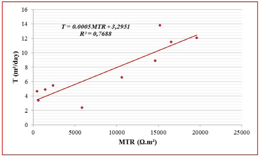
Figure 4 T expressed as a function of MTR in order to establish an empirical relationship between both parameters.
With R 2 = 0.7688
Equation 10 will be used to extrapolate T values at the remaining 36 VES points where no water sample exists.
Extrapolation of T in the whole region
In order to estimate MTR values in the remaining 36 VES points without water sample, the formula established in equation (7) is applied. Equation 8 is thereafter used to compute K values in those VES without water sample. In other terms, since the transverse resistance of each point is known (as the product of rock resistivity by its thickness as expressed by earlier Equation 5) from VES interpretation, the empirical relationship established in Equation 7 enables us to obtain the modified transverse resistance as the product of the transverse resistance by 0.8518 plus 1005.6. Finally, the transmissivity of each point is obtained as the product of the modified transverse resistance by 5 × 10⁻⁴ plus 3.2951. This methodology takes into account the geological context of the study area as exposed in Section 3.
Results and discussion
This geoelectrical investigation consisted in applying the approach developed and proposed recently by Asfahani (2016) on 14 reference VES, then using the above calibrated relationships established to extrapolate aquifer parameters in the whole study area. Two relationships have been established: one between MTR and TR ( Equation 7), and another between T and MTR ( Equation 8). Those relationships were established assuming that the study area is geologically homogeneous and regular.
Hydrogeophysical parameters of 14 reference VES
Fourteen VES were conducted near existing boreholes with available water samples. Interpretation of those VES enabled to compute rock resistivity (ρrock) and aquifer thickness (h) at those points. The corresponding transverse resistance (TR), modified transverse resistance (MTR), formation factor (F) and hydraulic conductivity (K) are thereafter computed since the expression of water resistivity (ρw) is known. These parameters are represented in Table 1.
Those 14 reference boreholes have an average value of water resistivity
Table 2 Averaged statistical hydraulic and geophysical parameters of the 14 reference VES points presented in Table 1.
| Parameter | Min | Max | Average |
|---|---|---|---|
| h (m) | 8.40 | 60.00 | 31.67 |
| ρ rock (Ω.m) | 28.00 | 565.00 | 229.05 |
| ρw(Ω.m) | 1.51 | 5.21 | 3.00 |
| F | 9.34 | 188.42 | 76.39 |
| TR (Ω.m2) | 330.40 | 22600.00 | 7021.17 |
| MTR (Ω.m2) | 447.54 | 19587.12 | 7486.57 |
| K (m/day) | 0.09 | 0.89 | 0.29 |
| T (m2/day) | 2.42 | 17.27 | 9.12 |
Hydrogeophysical parameters of 36 remaining VES without available water sample
MTR ant T at the 36 VES points without available water samples are obtained using the established empirical Equations 7 and 8. The resulting MTR, T, and K values enable to approximately characterize the Pan-African aquifer. Those values are presented and compared with previous results (Arétouyap et al., 2015) as shown in Table 3. Significant changes between those results are visible in hydraulic conductivity and transmissivity values. This difference attests the necessity and the advantage of using this alternative approach, where salinity variations from place to place are taken into consideration.
Table 3 Hydrological and geophysical parameters of the 36 VES points without available water samples, in comparison with previous results (Arétouyap et al., 2015).
| VES | h (m) | ρ (Ω.m) | TR (Ω.m2) | MTR (Ω.m2) | T (m2/day) | T* (m2/day) | K (m/day) | K*(m/day) |
|---|---|---|---|---|---|---|---|---|
| P-1 | 25 | 811.0 | 20275.0 | 18775.85 | 12.68 | 26.62 | 0.51 | 1.06 |
| P-2 | 47 | 362.1 | 17018.7 | 16002.13 | 11.30 | 39.25 | 0.24 | 0.84 |
| P-4 | 48 | 175.7 | 8433.6 | 8689.34 | 7.64 | 8.09 | 0.16 | 0.17 |
| P-5 | 20 | 608.0 | 12160.0 | 11863.49 | 9.23 | 16.93 | 0.46 | 0.85 |
| P-6 | 6 | 157.0 | 942.0 | 2308.00 | 4.45 | 10.06 | 0.74 | 1.68 |
| P-7 | 10 | 137.0 | 1370.0 | 2672.57 | 4.63 | 0.09 | 0.46 | 0.09 |
| P-10 | 19 | 114.1 | 2167.9 | 3352.22 | 4.97 | 28.40 | 0.26 | 1.49 |
| P-11 | 40 | 410.0 | 16400.0 | 15475.12 | 11.03 | 48.60 | 0.28 | 1.21 |
| P-12 | 37 | 22.0 | 814.0 | 2198.97 | 4.40 | 43.25 | 0.12 | 1.17 |
| P-14 | 8 | 8.0 | 64.0 | 1560.12 | 4.08 | 1.87 | 0.51 | 0.23 |
| P-18 | 43 | 408.0 | 17544.0 | 16449.58 | 11.52 | 38.71 | 0.27 | 0.90 |
| P-19 | 34 | 26.0 | 884.0 | 2258.59 | 4.42 | 6.91 | 0.13 | 0.20 |
| P-20 | 61 | 188.0 | 11468.0 | 11274.04 | 8.93 | 13.76 | 0.15 | 0.23 |
| P-21 | 19 | 221.5 | 4208.5 | 5090.40 | 5.84 | 42.63 | 0.31 | 0.55 |
| P-24 | 17 | 112.9 | 1919.3 | 3140.46 | 4.87 | 3.29 | 0.29 | 0.33 |
For each VES point presented in Table 3, the K* value of the hydraulic conductivity can be obtained as a ratio of the transmissivity T to the saturated thickness h obtained at that point. The spatial distribution of h is shown in Figure 5, where its values range from 6 to 84 m, with an average of 32 m.

The spatial distribution of the transverse resistance (TR) shown in Figure 6 reveals that TR values range from 330 to 22600 Ω.m2 with an average value of 7021 Ω.m2.

The distributions of the modified transverse resistance (MTR), transmissivity (T) and hydraulic conductivity (K) are also shown respectively in Figures 7, 8 and 9, and summarized in Table 4. Many similitudes are observed between TR distribution (Figure 6) and MTR distribution (Figure 8). Respective minimum and maximum values are located in the same regions. However, one can observe a minor dissimilarity in the variation rate and direction. This change can be explained by several factors as electric anisotropy, mineralogical variation, hydraulic anisotropy and lithological disparity. Furthermore, since the local aquifer results from the bedrock alteration/weathering, it is possible to have many mini aquifers confined in unconnected aquitards.


Table 4 Statistical hydraulic and geophysical parameters of the 36 VES points without available water samples.
| Parameter | Min | Max | Average | SD |
|---|---|---|---|---|
| h (m) | 6 | 98 | 32.08 | 21.49 |
| ρ rock (Ω.m) | 3 | 825 | 225.21 | 222.18 |
| TR (Ω.m2) | 24 | 31350 | 7476.20 | — — |
| MTR (Ω.m2) | 1526.04 | 28209.53 | 7873.83 | 6844.31 |
| K (m/day) | 0.07 | 0.74 | 0.31 | 0.17 |
| T (m2/day) | 4.06 | 17.40 | 7.23 | 3.42 |
| TR (Ω.m2) | 24 | 31350 | 7476.20 | — — |
| MTR (Ω.m2) | 1526.04 | 28209.53 | 7873.83 | 6844.31 |
The transmissivity distribution shown in Figure 9 exhibits the existence of a poor-transmissive zone in the eastern part of the study area. Transmissivity values are low in this area contrary to the west and the center, where values can reach 17 m2/day. The presence of sedimentary formations can explain the easy spread of water in horizontal direction unlike the western area, covered by surficial granite.
However, it is important to note that hydraulic conductivity K varies in the opposite sense to transmissivity. Indeed, higher K values are observed eastward while lower ones are observed westward (Figures 8 and 9). This distribution can also be explained by the geological and lithological setting as in transmissivity distribution. On the other hand, the inverse proportion between hydraulic conductivity (derived from vertical flow) and transmissivity (derived from horizontal) can be due to the presence of vertical faults and lineaments in the region.
Transmissivity and hydraulic conductivity of the Pan-African aquifer are determined through the proposed alternative approach (Asfahani, 2016). However, the application of this approach recommends the respect of three fundamental principles:
Where there are water samples (the case of 14 reference VES points presented in Table 1), the hydraulic conductivity K is firstly estimated by such an alternative approach, while the transmissivity T is secondly computed by assuming an average constant hydraulic conductivity and a variable thickness h of the saturated aquifer.
Where there are no available water samples (e.g. 36 VES presented in Table 3), the transmissivity is firstly estimated by the proposed approach, while the hydraulic conductivity is secondly computed.
A field hydrogeological investigation should be conducted in order to estimate the uncertainty and the confidence level of this new proposed approach in the study area.
The first two rules are followed. In addition, the results obtained are compared with those of Arétouyap et al. (2015). This comparison shows a fairly good agreement between the values of the aquifer thickness and a slight agreement regarding the values of hydraulic conductivity and transmissivity (Figure 10). Those differences are due to the basis of the analysis method. In the previous study, Arétouyap et al. (2015) used an empirical linear relationship between Kσ and the resistance R of the aquifer, where K and σ represent the hydraulic conductivity and the electrical conductivity of the aquifer respectively. Yet in the present investigation, the aquifer hydraulic conductivity is the ratio of the transmissivity to the saturated thickness. Note that transmissivity values are derived from modified transverse resistance computed thanks to an empirical relationship between MTR and T. Furthermore, the present study has increased the number of reference boreholes, top to 14.

Discussion
Validation of the approach
The equation used to determine hydrodynamic parameters from this approach isan empirical relationship (Table 3). In order to assess its reliability, the values of transmissivity obtained experimentally from pumping tests and those computed analytically using equation 8, as shown in Table 5, we compared.
Table 5 Comparison of analytical and experimental values for the 14 existing boreholes.
| VES | T (m/day) | T# (m/day) | MTR (Ω.m2) |
|
|---|---|---|---|---|
| P-3 | 2.42 | 6.22 | 5856.52 | 1.57 |
| P-8 | 12.38 | 5.99 | 5382.48 | 0.52 |
| P-9 | 5.47 | 4.47 | 2353.97 | 0.18 |
| P-13 | 13.82 | 10.88 | 15164.20 | 0.21 |
| P-15 | 4.89 | 4.01 | 1435.20 | 0.18 |
| P-16 | 13.24 | 5.39 | 4201.97 | 0.59 |
| P-17 | 8.92 | 10.59 | 14597.97 | 0.19 |
| P-22 | 6.62 | 8.59 | 10593.60 | 0.29 |
| P-23 | 4.67 | 3.52 | 447.54 | 0.25 |
| P-26 | 10.94 | 6.23 | 5872.18 | 0.43 |
| P-31 | 11.51 | 11.56 | 16528.71 | 0.003 |
| P-33 | 12.09 | 13.09 | 19586.12 | 0.08 |
| P-39 | 3.39 | 3.59 | 604.10 | 0.06 |
| P-40 | 17.27 | 4.39 | 2187.41 | 0.75 |
| Average | 0.38 |
# Analytical values obtained from the empirical equation 9
This comparison shows an absolute random ranging from 0.003 to 1.576 with an average value of 0.38, which is bearable. Thus, this method that has already been proven inthe Quaternary and Paleogene aquifers in the semi-arid Khanasser valley region of Northern Syria (Asfahani, 2016) can also be used in the Pan-African context.
Further conditions on the approach
Since VES results are highly influenced by electrical noise, land use and other economic activities such as agriculture, livestock, tannery etc., measurements may be carried out in locations far away from any electrical line from several anthropogenic activity centers. K values are generally influenced. In order to mitigate such negative impacts, VES measurements may be calibrated and their 1D quantitative interpretation must necessarily reflect the aquifer lithology. This is the case of VES measurements presented in the present study. Geostatistical analysis largely contributes in assuming that VES data are not influenced by electrical noise.
Contamination is another technical concern. The methodology proposed by Asfahani (2016) and applied in this paper is entirely based on water resistivity. Any contamination of that water may affect and modify its resistivity, and by consequence will affect the K values. This methodology must therefore be applied in a proper area, without any contamination influence. If this is not the case, the contamination factor and its influence on water resistivity must be calibrated and moved away. Fortunately, our study area is free of any relevant contamination.
Conclusions
The transmissivity (T) and the hydraulic conductivity (K) of the Pan-African aquifer in the region of Adamawa-Cameroon have been determined using an alternative method based on VES interpretation. 14 experimental VES conducted in the vicinity of existing boreholes with known water resistivity are interpreted using curve matching method. This interpretation led to two mathematical laws (empirical equations). The first equation establishes a strong relationship between the modified transverse resistance (MTR) while the second links the transmissivity (T) to MTR. From those equations, aquifer of the study is characterized as follows: TR ranges from 24 to 31350 Ω.m2 with an average of 7476 Ω.m2; MTR ranges from 1526 to 28209 Ω.m2 with an average of 7476 Ω.m2; T ranges from 4 to 17.4 m2/day with an average of 7.23 m2/day; and K ranges from 0.07 to 0.74 m/day with an average of 0.31 m/day. A cross validation, comparing T values obtained respectively from pumping test and developed approach (Table 5) reveals a fairly agreement between both sets of values. This approach is then suitable for investigation in the Pan-African context extended from Africa to South America.

