


 nueva página del texto (beta)
 Inglés (pdf)
 Artículo en XML
 Referencias del artículo
 Enviar artículo por email
 Citado por SciELO
  Similares en
SciELO
Similares en
SciELO 
 Permalink
PACS: 21.45.-v; 25.10.+s; 11.80.Jy
1. Introduction
Strange nuclear physics is a very topical subject. The hyperon-nucleon (YN) and hyperon-hyperon (YY) interactions constitute the input for microscopic calculations of few- and many-body systems involving strangeness, such as exotic neutron star matter 1,2,3,4,5 or hypernuclei 6,7,8. There are theoretical debates 9,10,11,12,13,14 on the possible existence of a neutral bound state of two neutrons and a
When a two-baryon interaction is attractive, if the system is merged with nuclear matter and the Pauli principle does not impose severe restrictions, the attraction may be reinforced. Simple examples of the effect of a third or a fourth baryon in two-baryon systems could be given. The deuteron, (I)J
P
= (0) 1+, is bound by 2.225 MeV, while the triton, (I)J
P
= (1/2)1/2+, is bound by 8.480 MeV, and the
In this paper, we review our recent studies of the three-body systems:
One should bear in mind how delicate is the few-body problem in the regime of weak binding, as demonstrated in Ref. 40 for the
The review is organized as follows. In Sec. 2 we describe the technical details to solve the three-body bound state Faddeev equations as well as the generalized Gaussian variational method used to look for bound states of the four-body problem. In Sec. 3 we construct the two-body amplitudes needed for the solution of the bound state three- and four-body problems. The results are presented and discussed in Sec. 4. Finally, in Sec. 5 we summarize our main conclusions.
2. The three- and four-body bound-state problems
In this section we outline the solution of the three- and four-body bound-state problems. We will restrict ourselves to configurations where all particles are in S-wave states. The three-body problem has been widely discussed in the literature and we refer the reader to Refs. 47,48,49 for a more detailed discussion. The Faddeev equations for a system with total isospin I and total spin J are,
where
Expanding the amplitude
where
with
The four-body problem has been addressed by means of the variational method, specially suited for studying low-lying states. The nonrelativistic hamiltonian is be given by,
where the potential
The variational wave function must include all possible spin-isospin channels contributing to a given configuration. For each channel s, the wave function will be the tensor product of a spin (
where
where the eigenvalues are obtained by a minimization procedure.
For the description of the four-body wave function we consider the Jacobi coordinates:
The total wave function should have well-defined permutation properties under the exchange of identical particles. The spin part can be written as,
where the spin of the two N’s (Y’s) is coupled to S 12 (S 34). Two identical spin-1/2 fermions in a S = 0 state are antisymmetric (A) under permutations while those coupled to S = 1 are symmetric (S). We summarize in Table I the corresponding vectors for each total spin together with their symmetry propertiesii
Table I. Spin basis vectors for all possible total spin states (S). The ’Symmetry’ column stands for the symmetry properties of the pair of identical particles.

The most general radial wave function with total orbital angular momentum L = 0 may depend on the six scalar quantities that can be constructed with the Jacobi coordinates of the system, they are:
where n is the number of Gaussians used for each spin-isospin component.
where P x and P y are -1 for antisymmetric states, (A), and +1 for symmetric ones, (S). Thus, one can build the following radial combinations, (P x P y ) = (SS), (SA), (AS), and (AA):
The last equations can be expressed in a compact manner by defining the following function,
and the vectors
and
which allows to write Eqs. (13)-(15) as,
The radial wave function includes all possible internal relative orbital angular momenta coupled to L = 0. It has also well-defined symmetry properties on the
To evaluate radial matrix elements we use the notation introduced in Eq. (19):
where
being
where we have shortened the previous notation according to
where the functions f (x, y, z) are the potentials. Being all of them radial functions (not depending on angular variables) one can solve the previous integral by noting:
where
One can extract some useful relations for the radial matrix elements using simple symmetry properties. Let us rewrite Eq. (21)
If f (x, y, z) depends only in one coordinate, for example
The radial wave function described in this section is adequate to describe not only bound states, but also it is flexible enough to describe states of the continuum within a reasonable accuracy 50,51,52.
3. Two-body amplitudes
We have constructed the two-body amplitudes for all subsystems entering the three- and four-body problems studied by solving the Lippmann-Schwinger equation of each (i, j) channel,
where
and the two-body potentials consist of an attractive and a repulsive Yukawa term, i.e.,
The parameters of the
Table II. Low-energy data and parameters of the local central Yukawa-type potentials given by Eq. (31) for the NN potential 54, and the most recent updates of the ESC08c Nijmegen interactions for the

a This channel is discussed on Sec. III.
The
The potentials obtained are shown in Fig. 1. In Fig. 1(a) we show the

Figure 1. (a)
4. Results and discussion
Let us first of all show the reliability of the input potentials. We compare in Fig. 2 the

Figure 2. (a)
The reasonable description of the known two- and three-body problems gives confidence to address the study of other three- and four-body systems. We show in Table III the channels of the different two-body subsystems contributing to each (I, J) three- and four-body state that we will study. For the
Table III. Two-body NN, YN and YY isospin-spin (i, j) channels that contribute to a given three- or four-body state with total isospin I and total spin J. The last column indicates the corresponding threshold for each state, that would come given by

4.1. Three-body systems
We show in Fig. 3 the Fredholm determinant of all
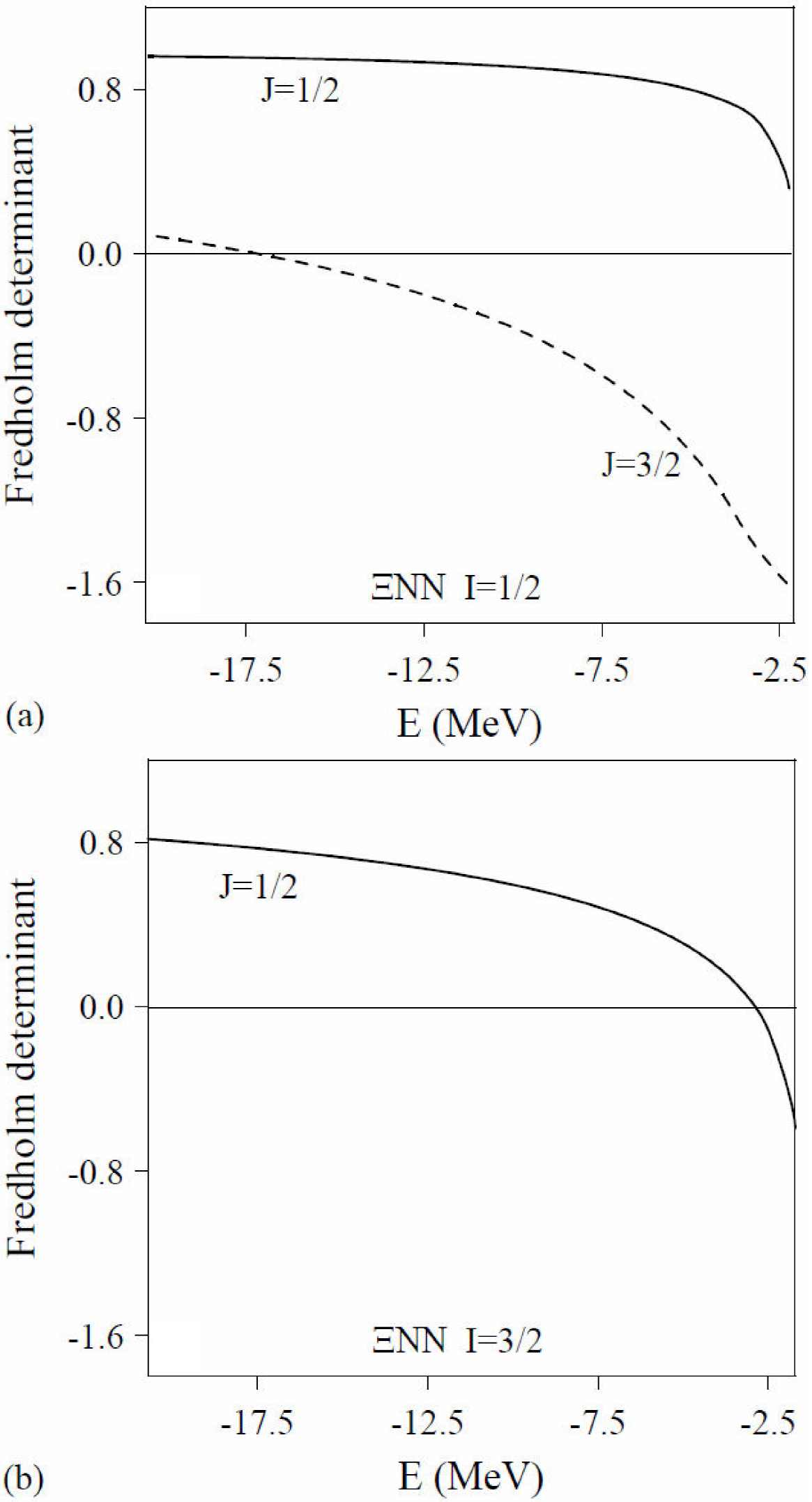
Figure 3. (a) Fredholm determinant for the J = 1/2 and J = 3/2 I = 1/2
For the
Thus, due to the negative sign in the r.h.s. the
Finally, we show in Fig. 4 the Fredholm determinant of all

Figure 4. (a) Fredholm determinant for the J = 1/2 and J = 3/2 I = 1/2
Let us finally mention that our results for three-body systems containing a
4.2. Four-body systems
In the previous section we have seen that all three-body systems made of N’s and
The binding energy of the

Figure 5. Binding energy of the (I)J
P
= (2)0+
One can also study the behavior of the root mean square radius (RMS) of the four-body system, defined in the usual way,
The results are shown in Fig. 6, where besides the RMS radius we have also calculated the root mean square radii of the different Jacobi coordinates. As seen in Table III, only the 1S0(I = 1) NN and

Figure 6. Root mean square radii of the (I)J
P
= (2)0+
We have finally evaluated the binding energy of the
We have studied the dependence of the binding on the strength of the attractive part of the different two-body interactions entering the four-body problem. For this purpose we have used the following interactions,
with the same parameters given in Table II. The system hardly gets bound for a reasonable increase of the strength of the the

Figure 7. Binding energy of the (I)J
P
= (1)0+ nn
Reference 14 tackled the same problem by fitting low-energy parameters of older versions of the Nijmegen-RIKEN potential 30,69 or chiral effective field theory 55,70, by means of a single Yukawa attractive term or a Morse parametrization. The method used to solve the four-body problem is similar to the one we have used in our calculation, thus the results might be directly comparable. Our improved description of the two- and three-body subsystems and the introduction of the repulsive barrier for the 1 S 0 NN partial wave, relevant for the study of the triton binding energy (see Table II of Ref. 71), leads to a four-body state just above threshold, that cannot get bound by a reliable modification in the two-body subsystems. As clearly explained in Ref. 14, the window of Borromean binding is more an more reduced for potentials with harder inner cores.
5. Summary
This manuscript intends to summarize our recent work on few-body systems made of N’s,

