SciELO - Scientific Electronic Library Online

 
vol.68 número4Initial value problem for a Caputo space-time fractional Schrödinger equation for the delta potentialAn empirical model for the Backscattering coefficient of 1-30 keV electrons from thin film targets índice de autoresíndice de materiabúsqueda de artículos
Home Pagelista alfabética de revistas  

Servicios Personalizados

Revista

Articulo

Indicadores

Links relacionados

  • No hay artículos similaresSimilares en SciELO

Compartir


Revista mexicana de física

versión impresa ISSN 0035-001X

Rev. mex. fis. vol.68 no.4 México jul./ago. 2022  Epub 19-Mayo-2023

https://doi.org/10.31349/revmexfis.68.040801 

Research

A non-renormalizable neutrino mass model with S3⊗Z2 symmetry

J. D. García-Aguilar1 

J. C. Gómez-Izquierdo1 

1Centro de Estudios Científicos y Tecnológicos No 16, Instituto Politécnico Nacional, Pachuca: Ciudad del Conocimiento y la Cultura, Carretera Pachuca Actopan km 1+500, San Agustín Tlaxiaca, Hidalgo, México. *e-mail: jdgarcia@ipn.mx; cizquierdo@ipn.mx


Abstract

The lepton sector is studied within a flavored non-renormalizable model where the S3⊗Z2 flavor symmetry controls the masses and mixings. In this work, the effective neutrino as well as the charged lepton mass matrices are hierarchical and these have (under a benchmark in the charged sector) a kind of Fritzsch textures that accommodate the mixing angles in good agreement with the last experimental data. The model favors the normal hierarchy, this also predicts consistent values for the CP-violating phase and the |mee| effective Majorana neutrino mass rate. Along with this, the branching ratio for the lepton flavor violation process, µ, is below the current bound.

Keywords: Neutrino mass and mixing; flavor symmetries

1. Introduction

In spite of the fact that Standard Model (SM) works almost perfectly, it fails to explain the neutrino experimental data, dark matter, baryon asymmetry of the universe and so forth1. Speaking about the mixings, the lepton sector exhibits a peculiar pattern which is totally different to the quark sector where the mixing matrix is almost diagonal and this puzzle remains unsolved.

In this line of thought, hierarchical quark mass matrices as the nearest neighbor interaction (NNI) textures2-5 and those that possess the generalized Fritzsch textures6, fit quite well the CKM matrix. In the lepton sector, according to the experimental data, the PMNS matrix has large values in its entries which can be explained by the presence of a symmetry behind the neutrino mass matrix. Currently, we can find in the literature elegant proposals (and their respective breaking) as the µ ↔ τ symmetry7 (see reference therein), µ ↔ τ reflection symmetry8-13, Tri-Bimaximal14-19, Cobimaximal mixing matrices20-25. Moreover, hierarchical mass matrices as the Fritzsch26 and the generalized Fritzsch textures6 also accommodate the PMNS mixing matrix.

The flavor symmetries27-30 have been useful to obtain textures in the fermion mass matrices and the corresponding mixing patterns. For example, the S3 discrete group has been studied in great detail in different scenarios31-48. In the mentioned literature there are few models49,50 where the Fritzsch textures have been implemented. Hence, the main purpose that we pursuit is to realize those textures by means the S3 flavor symmetry however we obtain a modified Fritzsch textures which are different to previous studies in the sense that there is an extra parameter in the lepton mass matrices. As a result of that, the theoretical mixing angles formulas come out distinct but their predictions are in accordance with experimental data.

Due to the last neutrino oscillations data seem to favor the normal hierarchy51, in this paper, we construct a non-renormalizable lepton model in the type II see-saw scenario where the S3⊗Z2 flavor symmetry controls the masses and mixings. We stress that the scalar sector of the mentioned model keeps intact so that flavons are included to generate the mixings. The effective neutrino as well as the charged lepton mass matrices are hierarchical and these have (under a benchmark in the charged sector) a kind of Fritzsch textures that accommodate the mixing angles in good agreement with the last experimental data. The model predicts consistent values for the CP-violating phase and the |mee| effective Majorana neutrino mass rate. Along with this, the branching ratio for the lepton flavor violation process, µ, is below the current bound.

The paper is organized as follows. The theoretical framework and matter content of the model are reviewed in section II, the flavored model is also described; we construct, in the section III, the PMNS mixing matrix and relevant features are pointed out. An analytical study is performed on the mixing angles expressions to find out the parameter space that fits the observables, this together with a numerical analysis in section IV. In section V, we give some model predictions and some interesting conclusions are shown in section VI.

2. The framework

We make a scalar extension of the SM that is based on the gauge group SU(3)C⊗SU(2)L⊗U(1)Y, however we will focus in the lepton sector so that the matter content is given by

L=νLeL1,2,-1,eR1,1,-2. (1)

In the scalar sector, we have

H=H+H01,2,1,Δ=Δ+2Δ++Δ0-Δ+21,3,2, (2)

where the Higgs triplet provides mass to the active neutrinos by means of the type II see-saw mechanism. In addition, three flavons, 𝜙(1,2,3), which are singlets under the gauge group, will generate the lepton mixings.

In this appealing framework, the Lagrangian can be read as

L=LSM-12YνL¯(iσ2)ΔLc-V(H,Δ,ϕ)+h.c, (3)

where the most general scalar potential, which is gauge invariant, is given by

V(H,Δ,ϕ)=mH2HH+12λH(HH)2+mΔ2Tr(ΔΔ)+12λΔ(Tr(ΔΔ))2+λHΔ(HH)Tr(ΔΔ)\na+λHΔ'HTΔH+mϕ2|ϕ|2+12λϕ|ϕ|4+λHϕ(HH)|ϕ|2+λΔϕTr(ΔΔ)|ϕ|2. (4)

We ought to remark that the flavor invariant scalar potential is not written explicitly because we are only interested in studying the masses and mixings. Nonetheless, let us address a brief comment for the flavons sector, according to the assignation given in Table I, the flavored invariant scalar potential can be mimicked by that one with three Higgs doublets as we can see in Refs.33,39,48. In here, we will just assume a vacuum expectation value (vev) alignment of the flavons, 〈𝜙〉I = v𝜙(1,0) and 〈𝜙3〉 = v𝜙3, that provide the mixings and this also reduce the free parameters in the lepton mass matrices. We emphasize that the mentioned vev’s alignment was obtained in a model with S3 symmetry and four Higgs doublets49; two of them (the other two) belong to a doublet (singlets) of S3, in fact the scalar potential for three and four Higgs doublets shares similar structures and features. Then, we would expect to obtain the same pattern for flavons if a detailed study of the scalar potential was made but this will leave out.

Table I Assignation under the S3⊗Z2. Here, I = 1, 2. 

Matter LI L3 eIR e3R 𝜙 I 𝜙3 H
S3 2 1S 2 1S 2 1S 1S 1S
Z2 1 1 1 1 -1 -1 -1 -1

Let us speak briefly on the flavor symmetry. As is well known, the S327 has three dimensional real representation that can be decomposed as 3S = 2⊕1S or 3 A = 2⊕1 A (the reader might see the Appendix A for details). This is key for getting hierarchical mass matrices. In addition, the Z 2 discrete symmetry can be used to forbid some Yukawa couplings.

2.1 The model

As we already commented, in the present model, the scalar sector contains one Higgs doublet (H) and one triplet (Δ) so that some flavons will be added to the matter content in order to generate the mass textures that provide the mixings. The full assignation, under the S3⊗Z2 for the matter fields, is given in Table I.

As one can notice, due to the Z2 symmetry there are no-renormalizable Yukawa mass term, then, at the next leading order in the cutoff scale we havei

-LY=y1eΛ[L¯1H(ϕ1e2R+ϕ2e1R)+L¯2H(ϕ1e1R-ϕ2e2R)]+y2eΛ[L¯1Hϕ3e1R+L¯2Hϕ3e2R]+y3eΛ[L¯1Hϕ1+L¯2Hϕ2]e3R+y4eΛL¯3[Hϕ1e1R+Hϕ2e2R]+y5eΛL¯3Hϕ3e3R+y1νΛ[L¯1iσ2Δ(ϕ1L2+ϕ2L1)+L¯2iσ2Δ(ϕ1L1-ϕ2L2)]+y2νΛ[L¯1iσ2Δϕ3L1+L¯2iσ2Δϕ3L2]+y3νΛ[L¯1iσ2Δϕ1+L¯2iσ2Δϕ2]L3+y4νΛL¯3[iσ2Δϕ1L1+iσ2Δϕ2L2]+y5νΛL¯3iσ2Δϕ3L3+h.c., (5)

as a consequence the lepton mass matrices have the following structure

Me=ae+be'becebeae-be'ce'fefe'ge, Mν=aν+bν'bνcνbνaν-bν'cν'cνcν'gν, (6)

with

ae=y2evϕ3Λ,be'=y1evϕ2Λ,be=y1evϕ1Λ,ce=y3evϕ1Λ,ce'=y3evϕ2Λ,fe=y4evϕ1Λ,fe'=y4evϕ2Λ,ge=y5evϕ3Λ,aν=y2νvΔϕ3Λ,bν'=y1νvΔϕ2Λ,bν=y1νvΔϕ1Λ,cν=y3νvΔϕ1Λ,cν'=y3νvΔϕ2Λ,gν=y5νvΔϕ3Λ. (7)

Since that neutrino mass matrix, that comes from the type II see-saw mechanism, is symmetric then y3ν=y4ν allows to understand the form of M V . On the other hand, v and v( stand for the vacuum expectation values (vev’s) of the Higgs doublet and triplet, respectively. To reduce free parameters in the lepton mass matrices, we assume the following vev’s pattern for the flavon doublet and singlet of S3, respectively: 〈𝜙〉 = v𝜙(1,0) and 〈𝜙3〉 = v𝜙3 ii . At the same time, we set the magnitudes of the vev’s as follows: v𝜙 ∼ λΛ and v𝜙3 λΛ wher λ = 0.225 is the Wolfenstein parameter. Before finishing this section, we would like to remark that the flavor symmetry is broken by the vev’s of the flavons and the cutoff Λ scale satisfies the hierarchy Λ >> v >> vΔ. Therefore, the main role that the flavons play is to provide the mixings as was already commented.

3. PMNS MIXING MATRIX

Due to the alignment, the mass matrices read as

Me=aebecebeae0fe0ge,Mν=aνbνcνbνaν0cν0gν. (8)

As one can notice, if ae (av) was zero, the charged lepton (neutrino) mass matrix would possess implicitly the NNI (Fritzschiii) textures. In general, the charged lepton mass matrix has five complex free parameters that can be reduced a little bit more by adopting the benchmark ce ≈ fe. As a result, the lepton mass matrices have the Fritzsch textures but the entry a(v,e) will modify slightly those textures, as we will show next.

The mixing matrices that take place in the PMNS matrix are obtained as follows. Me and Mv are diagonalized respectively by Ue(L,R) and Uv such that UeLMeUeR=M^e and UνMνUν*=M^ν where M^(e,ν)=Diag.(m(e,1),m(μ,2),m(τ,3)) contains the physical lepton masses. Then, we write Ue(L,R)=S12ue(L,R) and Uν=S12uν so that ueLmeueR=M^e and uνmνuν*=M^ν. Here, m and S12 can be read as

ml=albl0blalcl0clgl,  S12=010100001, (9)

where ℓ = v, e.

We can observe that m can be written as

ml=al13×3+0bl0bl0cl0clgl-al. (10)

Notice that the second mass matrix has the Fritzsch texture but the there is a shift due to the a parameter. Consequently, we expect a deviation to the Fritzsch prediction on the mixings. To see this, let us diagonalize the mass matrix, m, where the CP violating phases are factorized as ml=Plm¯lPl where

Pl=eiηl1000eiηl2000eiηl3,m¯l=|al||bl|0|bl||al||cl|0|cl||gl|. (11)

The above matrix, m¯l, is obtained with the following conditions

ηl1=arg(al)2,ηl2=arg(al)2,ηl3=arg(gl)2,ηl1+ηl2=arg(bl),ηl2+ηl3=arg(cl). (12)

The CP violating phase can be absorbed in the lepton fields by choosing properly the following matrices u 𝑒𝐿 = P 𝑒 O 𝑒 , u 𝑒𝑅 = P 𝑒 † O 𝑒 and u 𝜈 = P 𝜈 O 𝜈 . Here, O ℓ is an orthogonal matrix that diagonalizes to m¯l, this is M^l=OlTm¯lOl, then we will obtain O and there are two cases for the neutrino sector, this is, the normal and inverted hierarchy.

3.0.1. Normal Hierarchy (NH)

For this case, the diagonalization procedure is valid for charged lepton and the active neutrinos (ℓ = e, v). Then considering M^l=OlTm¯lOl, three free parameters of m ℓ can be fixed in terms of the physical masses and unfixed one free parameter, |a|, by means of the invariants of the m¯l: tr(m¯l), tr(m¯l2) and det(m¯l). Explicitly, we get

|gl|=ml3-|ml2|+ml1-2|al|,|bl|=(ml3-|al|)(|ml2|+|al|)(ml1-|al|)ml3-|ml2|+ml1-3|al|,|cl|=(ml3+ml1-2|al|)(ml3-|ml2|-2|al|)(|ml2|-ml1+2|al|)ml3-|ml2|+ml1-3|al|, (13)

where mℓ2 = -|mℓ2| in order to obtain real parameters. In addition, those must satisfy the constraint mℓ3 > |mℓ2| > mℓ1 > |a| > 0. Having fixed some matrix elements, the eigenvectors of m¯l are given by

Xi=1Ni|bl||cl|mli-|al||cl|mli-|al|2-|bl|2,withXiTXi=1. (14)

Here, N and mℓi are normalization factors and the physical masses, respectively. Along with this, the normalization factors N can be fixed by the condition XiTXi=1 that has to satisfy the eigenvectors. Consequently, the columns of O are given bye the eigenvectors of m¯l, this means O = (X1, -X2, X3).

After a lengthy task, we obtain

Ol=(m̃l2+ãl)(1-ãl)M2D1-(m̃l1-ãl)(1-ãl)M1D2(m̃l2+ãl)(m̃l1-ãl)M3D3(m̃l1-ãl)M2DD1(m̃l2+ãl)M1DD2(1-ãl)M3DD3-(m̃l1-ãl)M1M3D1-(m̃l2+ãl)M2M3D2(1-ãl)M1M2D3, (15)

with

M1=1+m̃l1-2ãl,M2=1-m̃l2-2ãl,M3=m̃l2-m̃l1+2ãl,D=1-m̃l2+m̃l1-3ãl,D1=(1-m̃l1)(m̃l2+m̃l1)D,D2=(1+m̃l2)(m̃l2+m̃l1)D,D3=(1+m̃l2)(1-m̃l1)D, (16)

where m̃l2=|ml2|/ml3, m̃l1=ml1/ml3 and ã = |a|/mℓ3. For simplicity, the mixing matrix elements have been normalized by the heaviest mass. Therefore, the constraint is replaced by 1>m̃l2>m̃l1>ãl>0.

3.0.2. Inverted Hierarchy (IH)

We want to remind you that this ordering is only valid for neutrinos, this means ℓ = v so that M^ν=OνTm¯νOν. Then, similarity to the normal case, one obtains

|gν|=m2-|m1|+m3-2|aν|,|bν|=(m3-|aν|)(|m1|+|aν|)(m2-|aν|)m2-|m1|+m3-3|aν|,|cν|=(|m1|-m3+2|aν|)(m2+m3-2|aν|)(m2-|m1|-2|aν|)m2-|m1|+m3-3|aν|, (17)

in this case, we choose m1 = -|m1| for getting real parameters. On the other hand, the eigenvectors have the same form as in Eq. (14) however the orthogonal matrix Ov is a little bit different due to the fact m1 = -|m1| so that Ov = (-X1, X2, X3). Therefore, the orthogonal real matrix is given by

Oν=-(1-ãν)(m̃3-ãν)N2Dν1(m̃1+ãν)(m̃3-ãν)N1Dν2(1-ãν)(m̃1+ãν)N3Dν3(m̃1+ãν)N2DνDν1(1-ãν)N1DνDν2(m̃3-ãν)N3DνDν3-(m̃1+ãν)N1N3Dν1(1-ãν)N2N3Dν2-(m̃3-ãν)N1N2Dν3, (18)

where

N1=m̃1-m̃3+2ãν,N2=1+m̃3-2ãν,N3=1-m̃1-2ãν,Dν=1-m̃1+m̃3-3ãν,Dν1=(1+m̃1)(m̃1+m̃3)Dν,Dν2=(1+m̃1)(1-m̃3)Dν,Dν3=(1-m̃3)(m̃1+m̃3)Dν, (19)

with m̃1=|m1|/m2, m̃3=m3/m2 and ãv = |av|/m2. Additionally, the neutrino masses and the free parameter ãv have to satisfy 1>m̃1>m̃3>ãν>0.

Hence, the PMNS mixing matrix is given by Vi=UeLUνi=OeTP¯eOνi with i = NH,IH. Along with this, P¯e=PePνDiag.(1,1,eiην) with (v = (v3 - ((.

Finally, the reactor, atmospheric and solar angles might be obtained by means the following expressions

sinθ13=|(Vi)13|=|(Oe)11(Oνi)13+(Oe)21(Oνi)23+(Oe)31(Oνi)33eiην|,sinθ23=|(Vi)23|1-sin2θ13=|(Oe)12(Oνi)13+(Oe)22(Oνi)23+(Oe)32(Oνi)33eiην|1-sin2θ13,sinθ12=|(Vi)12|1-sin2θ13=|(Oe)11(Oνi)12+(Oe)21(Oνi)22+(Oe)31(Oνi)32eiην|1-sin2θ13.(20)

Let us remark that |ae|, |av| and ηv are free parameters to be constrained. Along with this, the lightest neutrino mass is also a free parameter. As a result of this, we end up having four unknown parameters.

Before closing this section, a brief comment on the Majorana phases will be added. We have considered the CP parities for the complex neutrino masses which means that these can be either 0 or (. Thus, for the normal and inverted ordering we have (m3, m2, m1) = (+, -, +) and (m3, m2, m1) = (+, +, -,), respectively. Those CP parities values ensure that the fixed parameters given in Eq. (13) and Eq.(17) are reals.

4. Results

4.1. Analytical study

The purpose of this analytical study is to find out the free parameter values that fit the mixing angles. To do so, two neutrino masses can be fixed in terms of the squared mass scales Δm212=m22-m12 and 𝛥 𝑚 31 2 = 𝑚 3 2 − 𝑚 1 2 (𝛥 𝑚 13 2 = 𝑚 1 2 − 𝑚 3 2 ) for the normal (inverted) hierarchy, and the lightest neutrino mass. This means explicitly

m3=Δm312+m12,m2=Δm212+m12,NH,m2=Δm132+Δm212+m32,m1=Δm132+m32, IH. (21)

In addition, the experimental data, that will be used in this analytical and numerical study, is given in the Table II

Table II Leptonic data51,52

Observable Experimental value
me(MeV) 0.5109989461 ± 0.0000000031
mµ(MeV) 105.6583745 ± 0.0000024
mτ(MeV) 1776.86 ± 0.12
Δm212/1 0-5 eV2 0.02200+0.069-0.062
Δm312/1 0-5 eV2 2.55+0.02-0.03(2.45+0.02-0.03)
sin2 Θ12 0.318 ± 0.16
sin2 Θ23 0.574 ± 0.14 (0.578+0.10-0.17)
sin2 Θ13 0.02200+0.069-0.062 (0.02225+0.064 -0.070)
δCP 194+24-22 (284+26-28)

In the current analysis, central values will be used for the normalized masses and there is a hierarchy among those, this is, m̃μ>m̃e/m̃μ>m̃e, m̃2>m̃1/m̃2>m̃1 (for normal ordering) and m̃1>m̃3/m̃1m̃3 (for inverted ordering); actually, for the last hierarchy we have m2 ( m1(1+Δm212/2m12), then m̃3m̃3/m̃1. Consequently, we get the following values m̃e2.9×10-4, m̃e/m̃μ4.8×10-3 and m̃μ5.9×10⁻². At the same time, for the neutrinos one obtains

NH

m̃12×10-2;m̃1m̃20.115,m̃20.173, (22)

where the particular 𝑚 1 ≈0.001 has been taken for this case.

IH

m̃30.195;m̃3m̃10.198,m̃11, (23)

with m3 ( 0.01. This value is consistent with the current mass ordering.

Notice that particular values for the lightest neutrino mass have been considered for the normal and inverted hierarchy. Thus, we will obtain approximately the matrices Oe and Ov for the normal and inverted ordering, then the mixing angles must be calculated in analytical way for different scenarios.

NH 1>m̃l2>m̃l1>ãl>0.

Case I: ãl0. In this limit, the Fritzsch textures are recovered and the orthogonal matrix is given by

Olm~l2(1-m~l2)(1-m~l1)(m~l2+m~l1)(1-m~l2+m~l1)-m~l1(1+m~l1)(1+m~l2)(m~l2+m~l1)(1-m~l2+m~l1)m~l2m~l1(m~l2-m~l1)(1-m~l1)(1+m~l2)(1-m~l2+m~l1)m~l1(1-m~l2)(1-m~l1)(m~l2+m~l1)m~l2(1+m~l1)(m~l2+m~l1)(1+m~l2)(m~l2-m~l1)(1-m~l1)(1+m~l2)-m~l1(m~l2-m~l1)(1+m~l1)(1-m~l1)(m~l2+m~l1)(1-m~l2+m~l1)-m~l2(m~l2-m~l1)(1-m~l2)(1+m~l2)(m~l2+m~l1)(1-m~l2+m~l1)(1-m~l2)(1+m~l1)(1-m~l1)(1+m~l2)(1-m~l2+m~l1). (24)

Case II: ãlm̃l1.

Ol10001-m̃l11+m̃l2m̃l2+m̃l11+m̃l20-m̃l2+m̃l11+m̃l21-m̃l11+m̃l2. (25)

IH (1>m̃1>m̃3>ãν>0).

Case I: ãν0.

Oν-m̃3(1+m̃3)(1+m̃1)(m̃1+m̃3)(1-m̃1+m̃3)m̃1m̃3(1-m̃3)(1+m̃1)(1-m̃3)(1-m̃1+m̃3)-m̃1(1-m̃1)(1-m̃3)(m̃1+m̃3)(1-m̃1+m̃3)m̃1(1+m̃3)(1+m̃1)(m̃1+m̃3)m̃1-m̃3(1+m̃1)(1-m̃3)m̃3(1-m̃1)(1-m̃3)(m̃1+m̃3)-m̃1(m̃1-m̃3)(1-m̃1)(1+m̃1)(m̃1+m̃3)(1-m̃1+m̃3)(1+m̃3)(1-m̃1)(1+m̃1)(1-m̃3)(1-m̃1+m̃3)-m̃3(m̃1-m̃3)(1+m̃3)(1-m̃3)(m̃1+m̃3)(1-m̃1+m̃3). (26)

Case II: ãνm̃3.

Oν0011-m̃31+m̃1m̃1+m̃31+m̃10-m̃1+m̃31+m̃11-m̃31+m̃10. (27)

Having obtained the above approximated matrices, let us obtain the mixing angles for two scenarios (both for the normal hierarchy) that seem to accommodate the observables.

Scenario A: If Oe and Ov were like Eq. (24), then the mixing angles would be

sinθ13m~2m~1(1-m~1m~2)+m~em~μm~2(1-m~2)-m~e1-m~2 eiην,sinθ23-m~em~μ m~2m~1(1-m~1m~2)+m~2(1-m~2)-m~μ1-m~2 eiην1-sin2θ13,sinθ12-m~1m~2(1-m~1m~2)+m~em~μ1-m~2+m~em~2(1-m~2) eiην1-sin2θ13, (28)

where the notable hierarchy in the charged lepton has been taken into account. In the above expressions, the reactor, atmospheric and solar angles are controlled by the ratio m̃e/m̃μ0.069, m̃20.41 and m̃1/m̃20.34, respectively. In order to enhance the angle values, the phase ηv must be near to π. In this way, we have that sinθ13 ≈ 0.06, sinθ23 ≈ 0.6 and sinθ12 ≈ 0.25. As result of this, the reactor and solar angle are not in the allowed experimental region with the neutrino masses values given in Eq. (22).

Scenario B: If Oe and Ov were like Eqs. (24) and (25) respectively, then the mixing angles would be

sinθ13m~2m~11-m~1m~2,sinθ231-m~e1+m~μm~2(1-m~2)-m~μ+m~e1+m~μ1-m~2 eiην1-sin2θ13,sinθ12m~1m~21-m~1m~21-sin2θ13. (29)

As one can notice, the reactor angle is tiny in comparison to the scenario A, the atmospheric and solar angle are handled by the m̃20.41 and m̃1/m̃20.34; the atmospheric angle value can be increased by allowing that the phase ηv must be π. Therefore, we obtain sinθ13 ≈ 0.016, sinθ23 ≈ 0.58 and sinθ12 ≈ 0.32.

To finish this section, let us add that one would expect changes in the mentioned scenarios when the lightest neutrino mass varies in its allowed region. Therefore, the numerical study will help us to discard one scenario.

4.2. Numerical study

To do the numerical analysis, we will be working with the following expressions

sin2θ13=sin2θ13(|ae|,|aν|,ην,mj),sin2θ23=sin2θ23(|ae|,|aν|,ην,mj),sin2θ12=sin2θ12(|ae|,|aν|,ην,mj), (30)

where mj with j = 1,3 represents the lightest neutrino mass for normal and inverted hierarchy, respectively.

Notice that the mixing angle expressions depend on the unknown parameters so that we will vary them in such a way that those satisfy their respective constraints. Taking into account the lightest neutrino mass, in the normal (inverted) ordering, we have 1>m̃2>m̃1>ãν>0 (1>m̃1>m̃3>ãν>0). Additionally, for each hierarchy, the lightest mass varies in the region 0 - 0.9 eV, the effective phase 2π ≥ (v ≥ 0 and the charged lepton parameter 1>m̃μ>m̃e>ãe>0. Having commented this, we request that our theoretical expressions satisfy the experimental bounds up to 3σ, this allows us to scan the allowed regions for the free parameters that fit with great accuracy the experimental results.

At the end of the day, we will obtain scattered plots for each observable as function of each unknown parameter. Subsequently, the Dirac (CP CP-violating phase and the effective Majorana neutrino mass are fitted and these are model predictions.

In the Fig. 1, we observe that there is a region (0.01 - 0.014 eV) for the lightest neutrino mass where the observables are in great according to the experimental results.

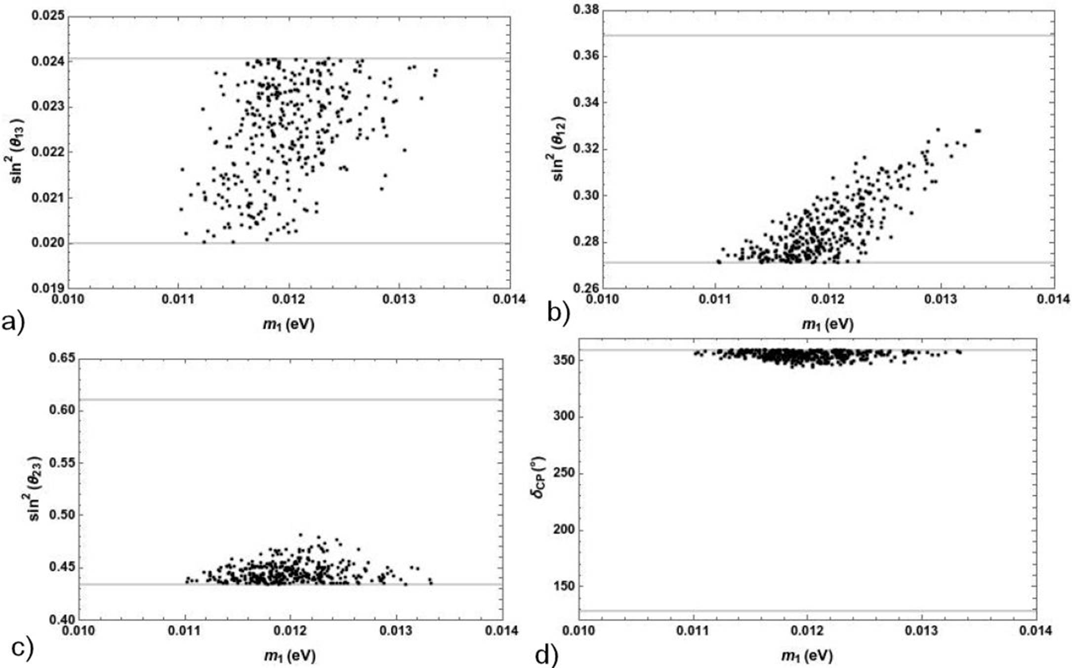
Figure 1 The reactor, solar, atmospheric angles and the Dirac CP phase as function of the lightest neutrino mass. The thick line stands for 3σ of C. L. 

According to the Fig. 2, the avv) prefers small values for fitting the mixing angles. This means the Fritzsch textures are favored but a small deviation is necessary to accommodate the observables up to 3σ.

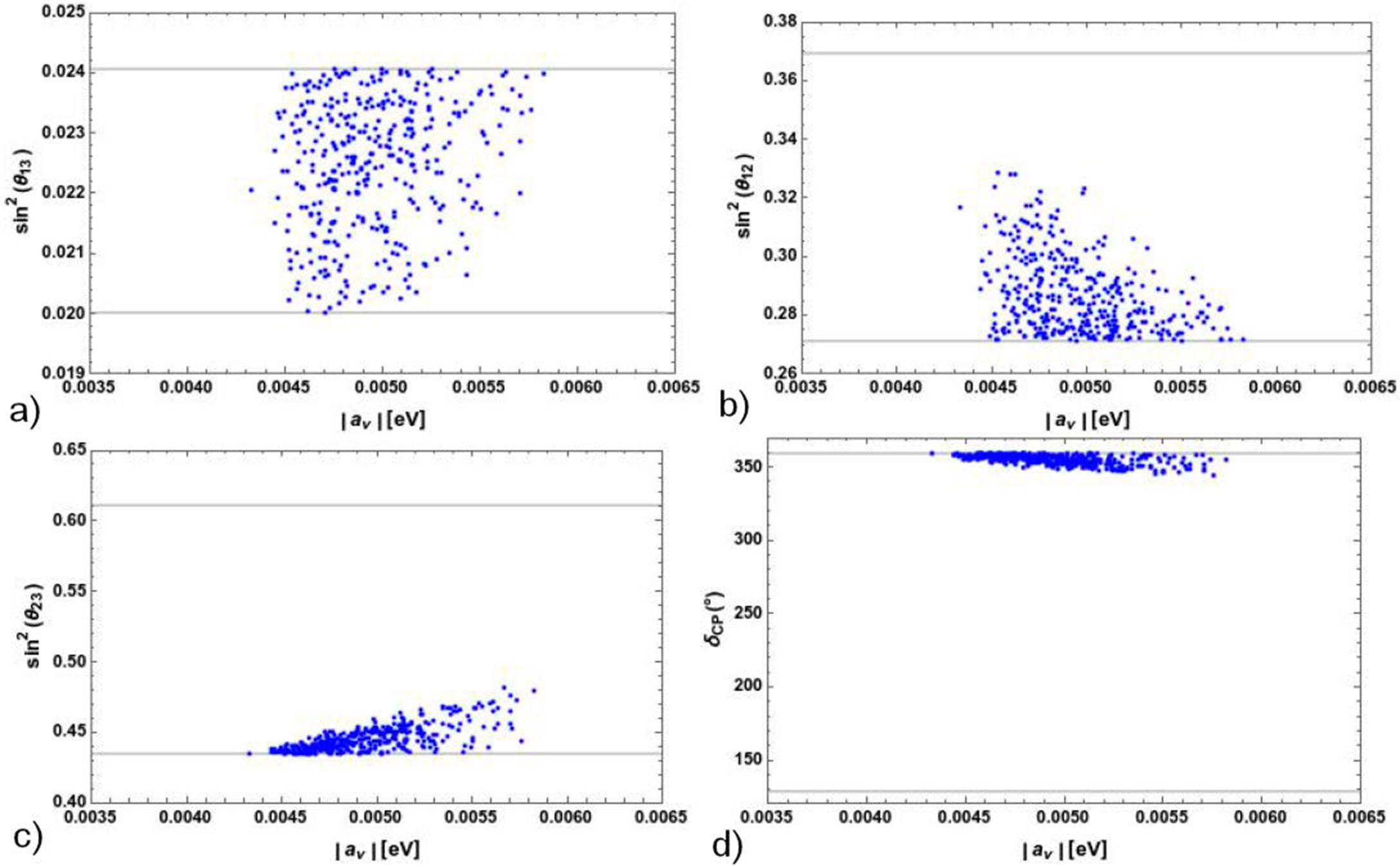
Figure 2 The reactor, solar, atmospheric angles and the Dirac CP phase as function of the |av| parameter. The thick line stands for 3σ of C. L. 

In the charged lepton sector, the aee) parameter region is close to the electron mass as can be seen in Fig. 3, this is, ae ≈ me, so that the observables are well accommodated in the scenario C. Let us focus in the ηv phase which lies in a region around π value, the full region is shown in the Fig. 4.

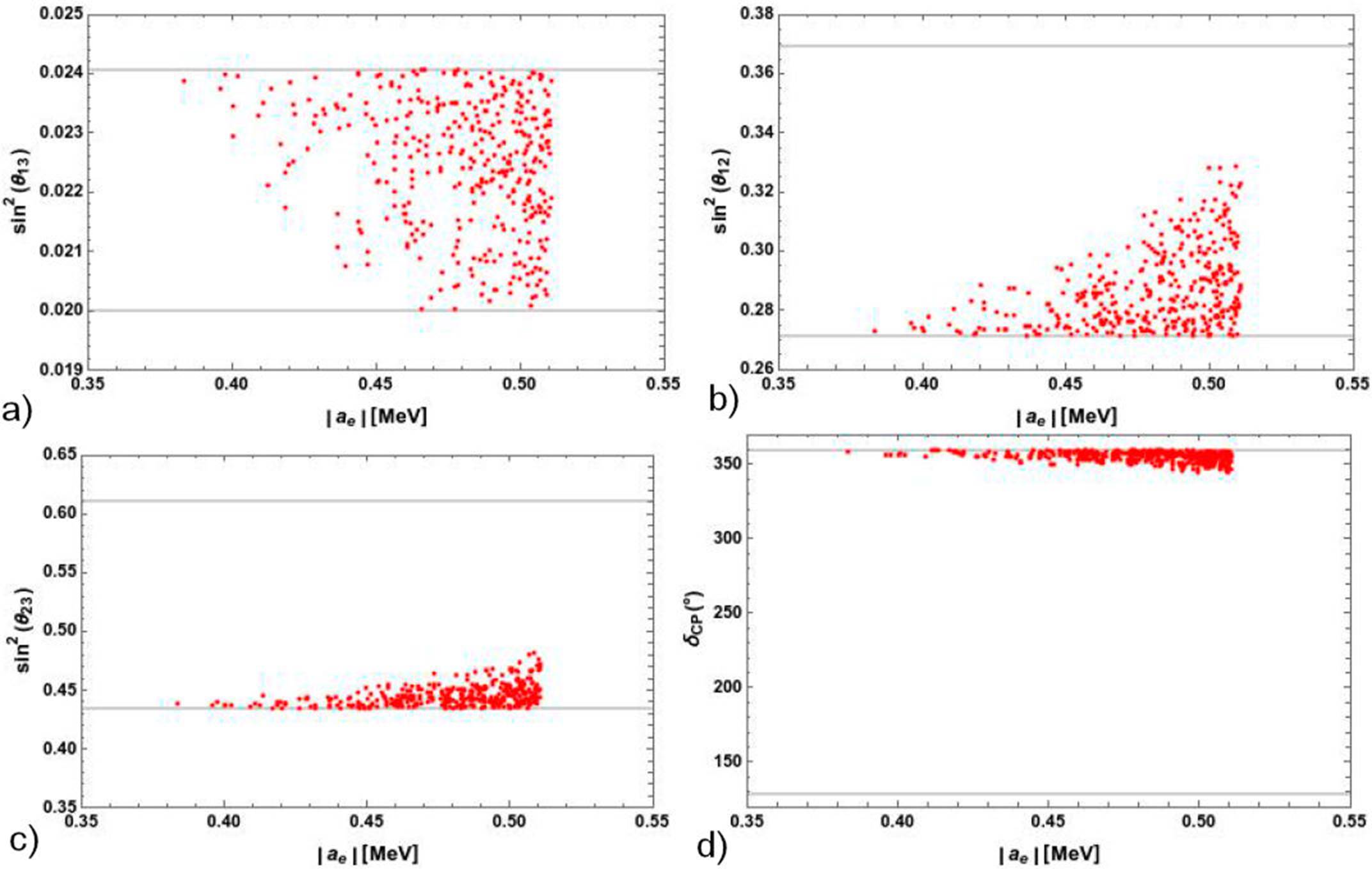
Figure 3 The reactor, solar, atmospheric angles and the Dirac CP phase as function of the |be| parameter. The thick line stands for 3σ of C. L. 

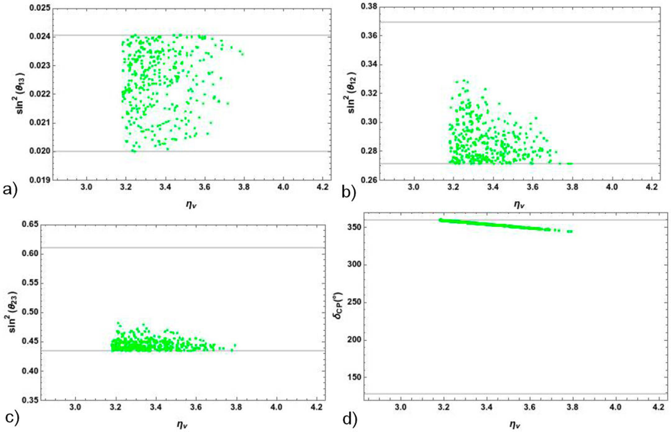
Figure 4 The reactor, solar, atmospheric angles and the Dirac CP phase as function of the effective phase, ηv, parameter. The thick line stands for 3σ of C. L. 

To summarize, a set of free parameters has been found in which the reactor, solar and the atmospheric angles can accommodate quite well but this latter lies in the allowed low region (3σ). In addition, the model predicts large values for the Dirac CP-violating phase which is close to the up region according to the experimental data.

5. Model Predictions

5.1. Effective Majorana neutrino mass rate

Going back to the comment about CP parities for the complex neutrino masses, we want to perform the effective Majorana mass of the electron neutrino, which is defined by

|mee|=|m1Ve12+m2Ve22+m3Ve32|, (31)

where mi and Vei (i = 1, 2, 3) are the complex neutrino masses and PMNS matrix elements. As it is well known, the lowest upper bound on |mee| < 0.22 eV was provided by GERDA phase-I data53 and this value has been significantly reduced by GERDA phase-II data54.

In the previous section, we found a set of values for the free parameters (see Figs. 1 to 4 which fit the mixing angles. As a result, those values were used to find the regions for the effective Majorana mass of the electron neutrino, as shown in the Fig. 5.

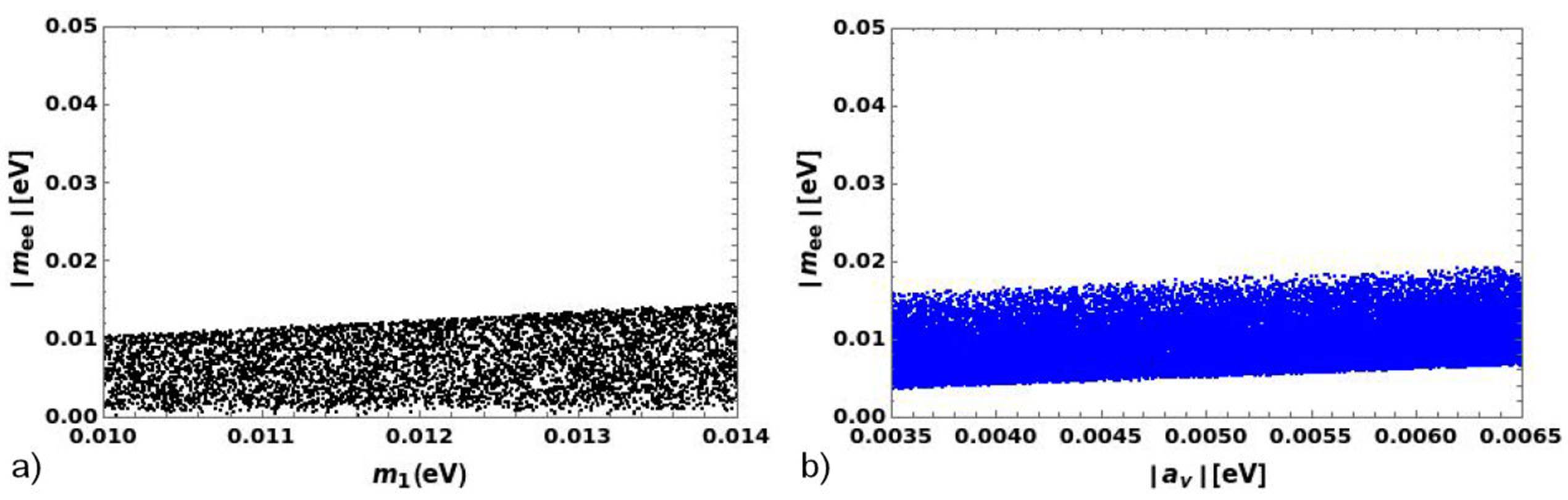
Figure 5 |mee| as function of m1 and |av|. These scattered plots correspond to the normal ordering where the CP parities for the complex neutrino masses are (m3, m2, m1) = (+, -, +). 

For this observable, two scattered plots have been only shown since that parameters m1 and av are more restrictive for the allowed region.

5.2. Lepton violation process: µ → eγ

As an immediate result, the branching ratio for the lepton flavor violation process µ → eγ55,56 may be performed. As is well known, the doubly (Δ++) and singly (Δ+) charged scalars, that come from the Higgs triplet (see Eq. (2)), mediate this process. The theoretical formula for the branching ratio55 can be written as

BR(μeγ)4.5×10-312vΔλ4V*M^νM^νVTeμ2200GeVmΔ++4, (32)

where we have assumed that the scalar masses, mΔ+ = mΔ++ ( mΔ, are degenerated. In here, V represents the PMNS mixing matrix.

In the previous section, we constrained the free parameters that fit the mixing angles, in good approximation, we obtained the following regions: 0.01 < m1 < 0.014 eV, 0.35 MeV > |ae| < me, 0.004 < |av| < 0.006 eV and π < ηv < 6π/5. Having done that, the branching ratio for the lepton flavor violation process µ → eγ can be calculated by using the values 80 GeV < mΔ and vΔ < 5 GeV for the single and doubly charged scalar masses and the vev of the Higgs triplet, respectively.

The allowed region for the branching ratio, as function of the vev of the Higgs triplet and the mass of the singly and doubly charged scalars, is exhibited in the Fig. 6. As one can realize, the model predicts a region that is too much below of the experimental bound BR(µ → eγ) ≈ 4.2 ( 10-13.

Figure 6 BR(µ → eγ) as function of vΔ and mΔ. The thick line stands for 3σ of C. L. 

6. Conclusions

We have built an economical non-renormalizable lepton model for getting the mixings where the type II see-saw mechanism is responsible to explain tiny neutrino masses. Under a particular benchmark, in the charged lepton sector, the mass matrices have the Fritzsch textures with a shift parameter which makes different to the previous studies. Our main finding is: a set of values for the relevant parameters was found to be consistent (up to 3σ) with the last experimental data on lepton observables for the normal neutrino mass ordering.

To finish, we would like to add that the S3⊗Z2 symmetry is an excellent candidate to be the flavor symmetry at low energy. However, one has to look for the best framework where the flavor symmetry solve the majority of open questions on the flavor problem and related issues. In this direction, the quark mixings and the scalar potential analysis will be included to have a complete study but this is a working progress.

Acknowledgements

García-Aguilar appreciates the facilities given by the IPN through the SIP project number 20211170. JCGI is supported by Project 20211423 and PAPIIT IN109321.

References

1. A. Masiero, S. K. Vempati and O. Vives, Flavour physics and grand unification, arXiv:0711.2903 [hep-ph]. [ Links ]

2. G. C. Branco, L. Lavoura and F. Mota, Nearest Neighbor Interactions and the Physical Content of Fritzsch Mass Matrices, Phys. Rev. D 39 (1989) 3443, https://doi.org/10.1103/PhysRevD.39.3443. [ Links ]

3. G. C. Branco and J. I. Silva-Marcos, NonHermitian Yukawa couplings?, Phys. Lett. B 331 (1994) 390-394, https://doi.org/10.1016/0370-2693(94)91069-3. [ Links ]

4. K. Harayama and N. Okamura, Exact parametrization of the mass matrices and the KM matrix, Phys. Lett. B 387 (1996) 614-622, https://doi.org/10.1016/0370-2693(96)01079-9. [ Links ]

5. K. Harayama, N. Okamura, A. I. Sanda and Z. Z. Xing, Getting at the quark mass matrices, Prog. Theor. Phys. 97 (1997) 781-790, https://doi.org/10.1143/PTP.97.781. [ Links ]

6. H. Fritzsch, Neutrino Masses and Flavor Mixing, Mod. Phys. Lett. A 30 (2015) 16 1530012, https://doi.org/10.1142/S0217732315300128. [ Links ]

7. Z. z. Xing and Z. h. Zhao, A review of (-( flavor symmetry in neutrino physics, Rept. Prog. Phys. 79 (2016) 7 076201, https://doi.org/10.1088/0034-4885/79/7/076201. [ Links ]

8. C. C. Nishi and B. L. Sánchez-Vega, Mu-tau reflection symmetry with a texture-zero, JHEP 01 (2017) 068, https://doi.org/10.1007/JHEP01(2017)068. [ Links ]

9. P. Chen, G. J. Ding, F. Gonzalez-Canales and J. W. F. Valle, Classifying CP transformations according to their texture zeros: theory and implications, Phys. Rev. D 94 (2016) 3 033002, https://doi.org/10.1103/PhysRevD.94.033002. [ Links ]

10. P. Chen, G. J. Ding, F. Gonzalez-Canales and J. W. F. Valle, Generalized (-( reflection symmetry and leptonic CP violation, Phys. Lett. B 753 (2016) 644-652, https://doi.org/10.1016/j.physletb.2015.12.069. [ Links ]

11. Z. h. Zhao, Breakings of the neutrino (-( reflection symmetry, JHEP 09 (2017) 023, https://doi.org/10.1007/JHEP09(2017)023. [ Links ]

12. Z. C. Liu, C. X. Yue and Z. h. Zhao, Neutrino (-( reflection symmetry and its breaking in the minimal seesaw, JHEP 10 (2017) 102, https://doi.org/10.1007/JHEP10(2017)102. [ Links ]

13. N. Nath, Z. z. Xing and J. Zhang, (-( Reflection Symmetry Embedded in Minimal Seesaw, Eur. Phys. J. C 78 (2018) 4 289, https://doi.org/10.1140/epjc/s10052-018-5751-y. [ Links ]

14. P. F. Harrison, D. H. Perkins and W. G. Scott, Tri-bimaximal mixing and the neutrino oscillation data, Phys. Lett. B 530 (2002) 167, https://doi.org/10.1016/S0370-2693(02)01336-9. [ Links ]

15. Z. z. Xing, Nearly tri bimaximal neutrino mixing and CP violation, Phys. Lett. B 533 (2002) 85-93, https://doi.org/10.1016/S0370-2693(02)01649-0. [ Links ]

16. G. Altarelli, F. Feruglio and L. Merlo, Tri-Bimaximal Neutrino Mixing and Discrete Flavour Symmetries, Fortsch. Phys. 61 (2013) 507-534, https://doi.org/10.1002/prop.201200117. [ Links ]

17. M. H. Rahat, P. Ramond and B. Xu, Asymmetric tribimaximal texture, Phys. Rev. D 98 (2018) 5 055030, https://doi.org/10.1103/PhysRevD.98.055030. [ Links ]

18. M. J. Pérez, M. H. Rahat, P. Ramond, A. J. Stuart and B. Xu, Stitching an asymmetric texture with Τ13×Z5 family symmetry, Phys. Rev. D 100 (2019) 7 075008, https://doi.org/10.1103/PhysRevD.100.075008. [ Links ]

19. M. H. Rahat, Leptogenesis from the Asymmetric Texture, Phys. Rev. D 103 (2021) 035011, https://doi.org/10.1103/PhysRevD.103.035011. [ Links ]

20. P. M. Ferreira, W. Grimus, D. Jurciukonis and L. Lavoura, Scotogenic model for co-bimaximal mixing, JHEP 07 (2016) 010, https://doi.org/10.1007/JHEP07(2016)010. [ Links ]

21. E. Ma, Soft A4 → Z3 symmetry breaking and cobimaximal neutrino mixing, Phys. Lett. B 755 (2016) 348-350, https://doi.org/10.1016/j.physletb.2016.02.032. [ Links ]

22. E. Ma and G. Rajasekaran, Cobimaximal neutrino mixing from A4 and its possible deviation, EPL 119 (2017) 3 31001, https://doi.org/10.1209/0295-5075/119/31001. [ Links ]

23. E. Ma, Cobimaximal neutrino mixing from S3×Z2, Phys. Lett. B 777 (2018) 332-334, https://doi.org/10.1016/j.physletb.2017.12.049. [ Links ]

24. W. Grimus and L. Lavoura, Cobimaximal lepton mixing from soft symmetry breaking, Phys. Lett. B 774 (2017) 325-331, https://doi.org/10.1016/j.physletb.2017.09.082. [ Links ]

25. A. E. Cárcamo Hernández and I. de Medeiros Varzielas, ((27) framework for cobimaximal neutrino mixing models, Phys. Lett. B 806 (2020) 135491, https://doi.org/10.1016/j.physletb.2020.135491. [ Links ]

26. H. Fritzsch, Texture zero mass matrices and flavor mixing of quarks and leptons, Mod. Phys. Lett. A 30 (2015) 28 1550138, https://doi.org/10.1142/S0217732315501382. [ Links ]

27. H. Ishimori, T. Kobayashi, H. Ohki, Y. Shimizu, H. Okada and M. Tanimoto, Non-Abelian Discrete Symmetries in Particle Physics, Prog. Theor. Phys. Suppl. 183 (2010) 1-163, https://doi.org/10.1143/PTPS.183.1. [ Links ]

28. W. Grimus and P. O. Ludl, Finite flavour groups of fermions, J. Phys. A 45 (2012) 233001, https://doi.org/10.1088/1751-8113/45/23/233001. [ Links ]

29. H. Ishimori, T. Kobayashi, H. Ohki, H. Okada, Y. Shimizu and M. Tanimoto, An introduction to non-Abelian discrete symmetries for particle physicists, Lect. Notes Phys. 858 (2012) 1-227, https://doi.org/10.1007/978-3-642-30805-5 [ Links ]

30. S. F. King and C. Luhn, Neutrino Mass and Mixing with Discrete Symmetry, Rept. Prog. Phys. 76 (2013) 056201, https://doi.org/10.1088/0034-4885/76/5/056201. [ Links ]

31. A. E. Cárcamo Hernández, I. de Medeiros Varzielas and E. Schumacher, Fermion and scalar phenomenology of a two-Higgs-doublet model with S3, Phys. Rev. D 93 (2016) 1 016003, https://doi.org/10.1103/PhysRevD.93.0160 [ Links ]

32. A. E. Cárcamo Hernández, R. Martinez and F. Ochoa, Fermion masses and mixings in the 3-3-1 model with right-handed neutrinos based on the S3 flavor symmetry, Eur. Phys. J. C 76 (2016) 11 634, https://doi.org/10.1140/epjc/s10052-016-4480-3. [ Links ]

33. D. Das and U. K. Dey, Analysis of an extended scalar sector with S3 symmetry, Phys. Rev. D 89 (2014) no.9, 095025 [erratum: Phys. Rev. D 91 (2015) 3 039905], https://doi.org/10.1103/PhysRevD.89.095025. [ Links ]

34. D. Das, U. K. Dey and P. B. Pal, S3 symmetry and the quark mixing matrix, Phys. Lett. B 753 (2016) 315-318, https://doi.org/10.1016/j.physletb.2015.12.038. [ Links ]

35. S. Pramanick and A. Raychaudhuri, Neutrino mass model with S3 symmetry and seesaw interplay, Phys. Rev. D 94 (2016) 11 115028, https://doi.org/10.1103/PhysRevD.94.115028. [ Links ]

36. D. Das, U. K. Dey and P. B. Pal, Quark mixing in an S3 symmetric model with two Higgs doublets, Phys. Rev. D 96 (2017) 3 031701, https://doi.org/10.1103/PhysRevD.96.031701. [ Links ]

37. J. C. Gómez-Izquierdo, Non-minimal flavored S3⊗Z2 left-right symmetric model, Eur. Phys. J. C 77 (2017) 8 551, https://doi.org/10.1140/epjc/s10052-017-5094-0. [ Links ]

38. E. A. Garcés, J. C. Gómez-Izquierdo and F. Gonzalez-Canales, Flavored non-minimal left-right symmetric model fermion masses and mixings, Eur. Phys. J. C 78 (2018) 10 812, https://doi.org/10.1140/epjc/s10052-018-6271-5. [ Links ]

39. J. C. Gómez-Izquierdo and M. Mondragón, BL Model with S3 symmetry: Nearest Neighbor Interaction Textures and Broken µ ↔ τ Symmetry, Eur. Phys. J. C 79 (2019) 3 285, https://doi.org/10.1140/epjc/s10052-019-6785-5 [ Links ]

40. D. Das and P. B. Pal, S3 flavored left-right symmetric model of quarks, Phys. Rev. D 98 (2018) 11 115001, https://doi.org/10.1103/PhysRevD.98.115001. [ Links ]

41. Z. Z. Xing and D. Zhang, Seesaw mirroring between light and heavy Majorana neutrinos with the help of the S3 reflection symmetry, JHEP 03 (2019) 184, https://doi.org/10.1007/JHEP03(2019)184. [ Links ]

42. S. Pramanick, Scotogenic S3 symmetric generation of realistic neutrino mixing, Phys. Rev. D 100 (2019) 3 035009, https://doi.org/10.1103/PhysRevD.100.035009. [ Links ]

43. A. Kunčinas, O. M. Ogreid, P. Osland and M. N. Rebelo, S3-inspired three-Higgs-doublet models: A class with a complex vacuum, Phys. Rev. D 101 (2020) 7 075052, https://doi.org/10.1103/PhysRevD.101.075052. [ Links ]

44. V. V. Vien, H. N. Long and A. E. Cárcamo Hernández, U(1) B-L extension of the standard model with S3 symmetry, Eur. Phys. J. C 80 (2020) 8 725, https://doi.org/10.1140/epjc/s10052-020-8318-7 [ Links ]

45. C. Espinoza, E. A. Garcés, M. Mondragón and H. Reyes-González, The S3 Symmetric Model with a Dark Scalar, Phys. Lett. B 788 (2019) 185-191, https://doi.org/10.1016/j.physletb.2018.11.028 [ Links ]

46. C. Espinoza and M. Mondragón, Prospects of Indirect Detection for the Heavy S3 Dark Doublet, arXiv:2008.11792 [hep-ph]. [ Links ]

47. V. V. Vien, 3 + 1 activesterile neutrino mixing in B-L model withcS3 × Z4 × Z2 symmetry for normal neutrino mass ordering, Eur. Phys. J. C 81 (2021) 5 416, https://doi.org/10.1140/epjc/s10052-021-09214-5 [ Links ]

48. M. Gómez-Bock, M. Mondragón and A. Pérez-Martínez, Scalar and gauge sectors in the 3-Higgs Doublet Model under the S3 symmetry, Eur. Phys. J. C 81 (2021) 10 942, https://doi.org/10.1140/epjc/s10052-021-09731-3. [ Links ]

49. D. Meloni, S. Morisi and E. Peinado, Fritzsch neutrino mass matrix from S3 symmetry, J. Phys. G 38 (2011) 015003, https://doi.org/10.1088/0954-3899/38/1/015003. [ Links ]

50. A. G. Dias, A. C. B. Machado and C. C. Nishi, An S3 Model for Lepton Mass Matrices with Nearly Minimal Texture, Phys. Rev. D 86 (2012) 093005, https://doi.org/10.1103/PhysRevD.86.093005 [ Links ]

51. P. F. de Salas, D. V. Forero, S. Gariazzo, P. Martínez-Miravé, O. Mena, C. A. Ternes, M. Tórtola and J. W. F. Valle, 2020 global reassessment of the neutrino oscillation picture, JHEP 02 (2021) 071, https://doi.org/10.1007/JHEP02(2021)071. [ Links ]

52. P. A. Zyla et al. [Particle Data Group], Review of Particle Physics, PTEP 2020 (2020) 8 083C01, https://doi.org/10.1093/ptep/ptaa104 [ Links ]

53. M. Agostini et al. [GERDA], Results on Neutrinoless Double-β Decay of 76Ge from Phase I of the GERDA Experiment, Phys. Rev. Lett. 111 (2013) 12 122503, https://doi.org/10.1103/PhysRevLett.111.122503. [ Links ]

54. M. Agostini, M. Allardt, A. M. Bakalyarov, M Balata, I. Barabanov, L. Baudis, C. Bauer, E Bellotti, S. Belogurov and S. T. Belyaev, et al., Background-free search for neutrinoless double-β decay of 76Ge with GERDA, Nature 544 (2017) 47, https://doi.org/10.1038/nature21717. [ Links ]

55. A. G. Akeroyd, M. Aoki and H. Sugiyama, Lepton Flavour Violating Decays tau → anti-l ll and mu → e gamma in the Higgs Triplet Model, Phys. Rev. D 79 (2009) 113010, https://doi.org/10.1103/PhysRevD.79.113010. [ Links ]

56. M. Lindner, M. Platscher and F. S. Queiroz, A Call for New Physics : The Muon Anomalous Magnetic Moment and Lepton Flavor Violation, Phys. Rept. 731 (2018) 1-82, https://doi.org/10.1016/j.physrep.2017.12.001. [ Links ]

57. A. E. Cárcamo Hernández, J. C. Gómez-Izquierdo, S. Kovalenko and M. Mondragón, ((27) flavor singlet-triplet Higgs model for fermion masses and mixings, Nucl. Phys. B 946 (2019) 114688, https://doi.org/10.1016/j.nuclphysb.2019.114688. [ Links ]

i The following Weinberg operators y6νΛL¯1cH2L1+L¯2cH2L2 and y7νΛL¯3cH2L3 are invariant under flavor and gauge symmetries nevertheless they are ignored and not included in the Lagrangian in Eq. (5) because their contributions are very small compared to av and gv due to the assumption of vev’s vΔ << v << Λ and v𝜙∼ v𝜙3 ≡ 〈𝜙3〉∼λΛ(, i.e., v2/( << vΔ 〈𝜙3〉/Λ.

ii In fact, one might consider two different vev’s alignments: (a) 〈𝜙〉 = v𝜙(0,1) and 〈𝜙3〉 = v𝜙3 but this does not provide the right mixings; (b) 〈𝜙〉 = v𝜙(1,1) and 〈𝜙3〉 = v3, in this case, the free parameters increase.

iii As is well known, the Fritzsch textures are given by

M=0A0A*0B0B*C. (A.2)

Appendix

A. S3 flavour symmetry

Several discrete flavor symmetries have been used in particle physics to face the flavor problem. In this line of thought, the non-Abelian group S327-30 has been explored in great detail with different purposes. In our case, due to its three dimensional representation can be decomposed as 3S = 2⊕1S or 3A = 2⊕1A, this allows us to get hierarchical mass matrices.

A complete study of the mentioned symmetry can be found in Refs.27-30, so that we just write multiplication rule between two doublets.

a1a22b1b22=(a1b1+a2b2)1S(a1b2-a2b1)1Aa1b2+a2b1a1b1-a2b22. (A.1)

Received: December 09, 2021; Accepted: January 14, 2022

Creative Commons License This is an open-access article distributed under the terms of the Creative Commons Attribution License