Introduction

The existence of multiple sources of uncertainty is a problem for risk management; this is the case when managing price and yield risks simultaneously. The former is represented by market risk and the latter by systematic risk. One way of managing price risk is using futures market hedging, cross hedge coverage such as that provided by the Agricultural Markets Commercialization and Development Services Agency (ASERCA in Spanish) (^{Martínez and García, 2010}). Another alternative is to impose a support price program (^{Martínez, 1990}); however this policy is no longer viable under current commercial treaties. With regard to systematic risk, this is more complicated, due to a number of factors such as weather or disease, which are uncertainty sources themselves. Thus, creating a multi-peril scheme is a limited solution because too many events need be covered (^{Goodwin, 1993}). Even without calamities, yield has a natural variation and that affects producer’s income. The motivation to manage price and yield risks is low because each of them offers only partial protection; the alternative is to manage income risk (^{Hennessy, 1998}). The main problem lies in the dependency between prices and yields when considering more than one planning point. To ensure an income, a risk-averse producer can be willing to pay a premium to get a minimum guaranteed income in case of price or yield variation. However, market conditions limit the possibilities to offer this kind of insurance because a number of non-independent risk sources have to be considered simultaneously. That is, insurance providers might not offer an income policy of this kind given the impossibility of modeling price and yield simultaneously. A price policy is itself difficult to operate because prices for the producers in one same area tend to move in the same direction; an insurance firm would need to have enough insured producers in different locations to buffer this problem. The same issue arises in yield insurance (^{Miranda, 1991}). In this case, yield can be affected by frost, flood, hail, plagues, or diseases. Given that each of these represent a risk source, it is more feasible to gather uncertainty under yield risk. The fact that there is a positive correlation for a delimited area is a problem.

Nonetheless, when managing agricultural risk the intention can be to ensure a minimum income, which involves price and yield uncertainty. The aim of this study was to model the dependency between price and yield for four of the main agricultural corn (Zea mays L.) producing states in Mexico. The dependency involves both the correlation between price and yield within each state and the correlation between prices and yields between different states. The hypothesis was that by modeling the dependency between price and yield income risk can be managed without resorting to two separate instruments -one for price and one for yield.

Materials and Methods

Prices and yields analyzed data correspond to the Mexican states of Sinaloa, Jalisco, Estado de México and Chiapas, on a yearly basis from 1980 to 2014; these states are the largest national corn producers (Sistema de Información Agroalimentaria de Consulta-Secretaría de Agricultura, Ganadería, Pesca y Alimentación; SIACON-SAGARPA^[2]). Each state has a variation both in price and yield, which depends on the technology employed and the intensity of inputs usage. In general, larger yields involve lower prices, except when producers can sell their products outside of the state. Besides, deciding to produce corn in a state can be influenced by prices and yields in other states. A producer’s income is the result of price time’s yield; in this study, income is considered to be what producers are interested in. The corn income per hectare produced within one state needs to include the dependency of price and yield and its dependency on other state’s prices and yields.

One way of modeling uncertainty sources is to use copula functions. These functions are used to model risk considering the price-yield dependency on Canadian barley and U.S. malt producers’ trade (^{Bekkerman et al., 2014}), in the agricultural insurance program assessment under different alternatives of copula functions (^{Goodwin y Hungerford, 2015}), and to calculate value at risk of a foreign exchange portfolio (^{Plascencia, 2012}). In each of these cases, modeling dependency between random variables and enhancing multivariate analysis is fundamental. In our study attention is drawn to dependency between price and yield by modeling income per hectare and thus managing the risk for that income.

A copula function is a p-variate joint distribution function which has uniform marginals (^{Nelsen, 2006}):

where C( ) has support defined in R^p over the hyperplane [0,1]^p and image defined in R¹ [0,1]; u_i denotes the uniform distribution over the [0,1] interval. If there are Y ₁, Y₂,... Y_p random variables with distribution functions F₁, F ₂,... F_p, and a joint distribution function F(Y₁, Y ₂,... Y_p), then if a copula function exists it will be such that:

If the copula function exists, it will be unique and can be obtained from:

An important property is that joint density can be represented as the product of the density of the copula by the product of the individual marginals:

From Skalar’s Theorem (^{Nelsen, 2006}) a copula’s density is defined as:

This highlights the fact that only with independent random variables the joint density can be factorized as the product of the corresponding marginals. However, there lies the practical importance of the copula functions, because the dependence can be model separately from the marginal distributions.

Results and Discussion

In our study, distributions were adjusted for the corresponding corn prices and yields for the states of Sinaloa, Jalisco, Estado de México and Chiapas, which amounts to eight random variables in total. The first issue that arises in this adjustment is that both prices and yields show trends, which moves the mean across time and this should be taken into account when adjusting a distribution. The trend in price is composed by inflation (which increases the mean), related goods’ effects, and imports’ effects of imports, which reduce the mean. Therefore, the trend was subtracted with a non-parametric algorithm that adjusts regression lines from a subset of data points close to the observed values iteratively; a detailed description can be found in ^{Cleveland et al. (1988)}. The advantage of this procedure is that it does not impose a particular prediction model, which eliminates the specification error while modeling data oscillation. The data used in the adjustment of price distributions where obtained as follows:

where y _t is the data used to adjust the marginal distributions; ŷ^p₂₀₁₄ is the predicted value for 2014 and εt^ is the residual of the non-parametric adjustment; the same treatment was performed on yield data. This implies treating the data as observed in 2014, considering the observed historic variations.

Using these trend free data, a distribution was adjusted to the price and the yield of each aforementioned state. Even after eliminating the trend, price remains a random variable and its variation is due to unexpected changes in input’s prices, related goods prices and imported corn prices, which are modeled under distribution function. Given that both prices and yields are positive values, a positive support set of distribution functions was used; a good fit was obtained under Wald, Gama and Beta distributions (^{Bekkerman et al., 2014}; ^{Goodwin y Kerr, 1988}). These distributions were used as marginals in the copula functions adjustment. The gaussian and t copulas were tested; these functions are appropriate when the nature of the dependency comes mainly from data around the mean, as would be expected for price and yield data.

Let u_j ~U(0,1) for j=1,2,...,m where m is the total amount of random variables used and U denotes the uniform distribution on the [0,1] interval; let Σ be a positive semidefinite correlation matrix, then the normal copula function can be written as:

where ^ΦΣ denotes the m-variate normal distribution function with mean a null vector and covariance matrix Σ and Θ^-1: denotes the inverse normal function. In this case, Σ is unknown, thus the adjustment consists in estimating that parametric matrix.

Let C_(ν,Σ) be the t copula function with ν ϵ(1,...,∞) and Σ be a correlation matrix, let t_ν be a univariate t distribution with zero mean and ν degrees of freedom, then the t copula can be written as:

where t_{(ν, Σ)} is a multivariate t distribution, with ν degrees of freedom and correlation matrix Σ, and t^-1_v(u_j) denotes the inverse t distribution with ν degrees of freedom. In this case what is unknown and must be solved by estimation are the correlation matrix and the degrees of freedom.

In each case, maximum likelihood estimation can be applied (^{Kjersti, 2004}; ^{McNell et al. 2015}), in the case of a normal copula only the correlation matrix is estimated, and in the case of a t copula the degrees of freedom must be estimated as well (^{Kjersti, 2004}; ^{McNell et al. 2015}). Estimating the corresponding correlation matrixes for the normal and t copulas allows verifying the negative correlation between price and yield especially within the same state, as can be observed for the states of Sinaloa, Estado de México and Chiapas (Table 1 and 2). In Jalisco’s case, the correlation between price and yield was positive, which would make for a risky income per hectare in that state. However, yield in Jalisco had a negative correlation with prices in Sinaloa, Estado de México and Chiapas under the normal copula function, and only with Sinaloa under the t copula.

Table 1 Correlation matrix estimated under the normal copula. 

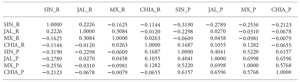
SIN_R: yield in Sinaloa; JAL_R: yield in Jalisco; MX_R: yield in Estado de Mexico; CHIA_R: yield in Chiapas; SIN_P: price in Sinaloa; JAL_P: price in Jalisco; MX_P: price in Estado de Mexico; CHIA_P: price in Chiapas.

Table 2 Correlation matrix estimated under the t copula. 

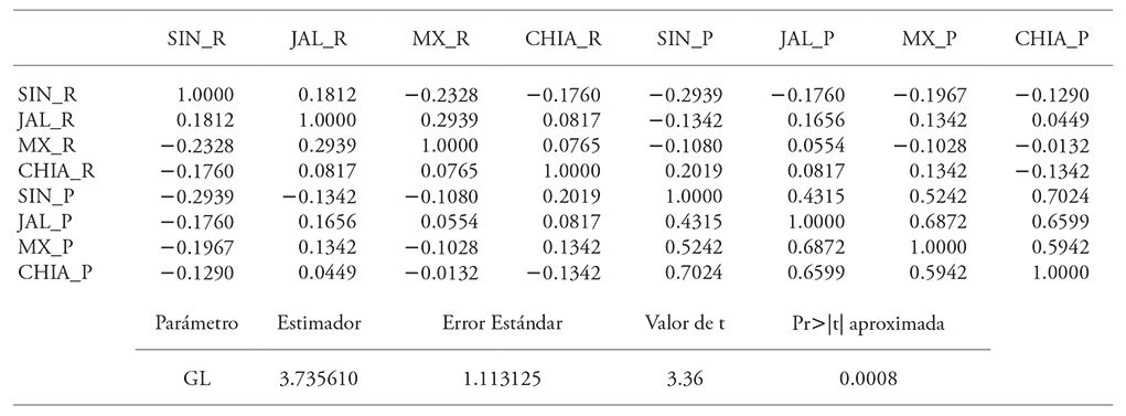
SIN_R: yield in Sinaloa; JAL_R: yield in Jalisco; MX_R: yield in Estado de Mexico; CHIA_R: yield in Chiapas; SIN_P: price in Sinaloa; JAL_P: price in Jalisco; MX_P: price in Estado de Mexico; CHIA_P: price in Chiapas.

This supports distributing income risk in a coverage scheme that includes producers in states other than Jalisco itself. In addition, price correlation between states is positive, which is the reason why it is necessary to search for negative correlations with yield within or outside the state to cover for price risk.

The correlation matrixes’ estimators differ due to the adjusted functional form in each case. Now, given the interest in a particular event such as:

Despite having the copula and marginal functions, it is not possible to obtain this probability by direct integration because the involved integral does not have an analytical closed form. One solution is to simulate a sample from the copula function and use the empirical marginals. Here values were simulated from the corresponding adjusted copula function; in particular, a random 1000 sample was generated out of the eight employed variables (four prices and four yields). This produces the eight synthetic variables with the estimated dependency structure. However, these variables are uniformly distributed. To return data to its original form, the inverse transformation was used:

where y is the random generated price or yield variable; F^-1( ) is the inverse function of the marginal distributions used; u is a uniform random variable obtained from the simulation of the copula function.

The advantage of this approach is that each simulated variable contains the within-state effect and the between-state effect simultaneously. Hence, these data can be treated as emerging from a joint distribution. In this case, data were used to model income per hectare -obtained as price times yield- for each of the four states.

Income per hectare can be built by calculating price’s and yield’s quantiles. This allows distinguishing income loss thresholds by state, which considers the joint price and yield dependency within and between states (Table 3 for the normal copula function, Table 4 for the t copula function).

Table 3 Price, yield quantiles and income claims under the normal copula function. 

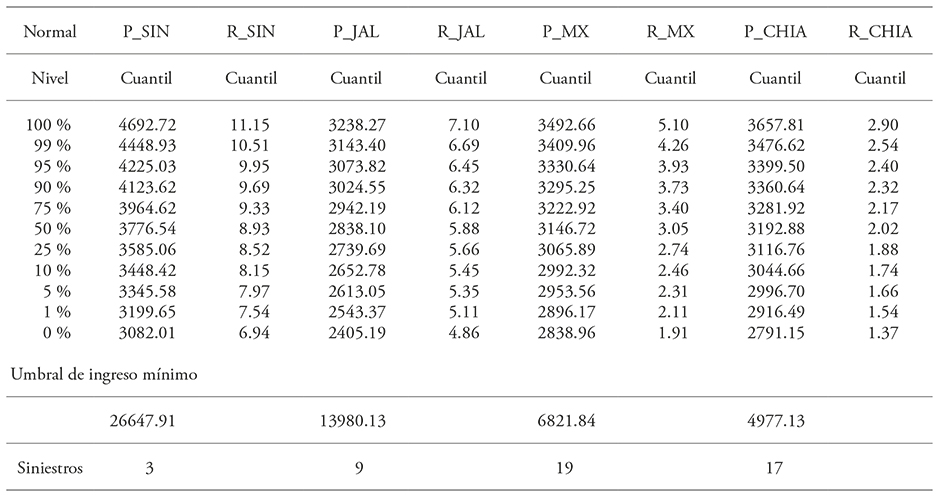
SIN_R: yield in Sinaloa; JAL_R: yield in Jalisco; MX_R: yield in Estado de Mexico; CHIA_R: yield in Chiapas; SIN_P: price in Sinaloa; JAL_P: price in Jalisco; MX_P: price in Estado de Mexico; CHIA_P: price in Chiapas.

Table 4 Price, yield quantiles and income claims under the t copula function. 

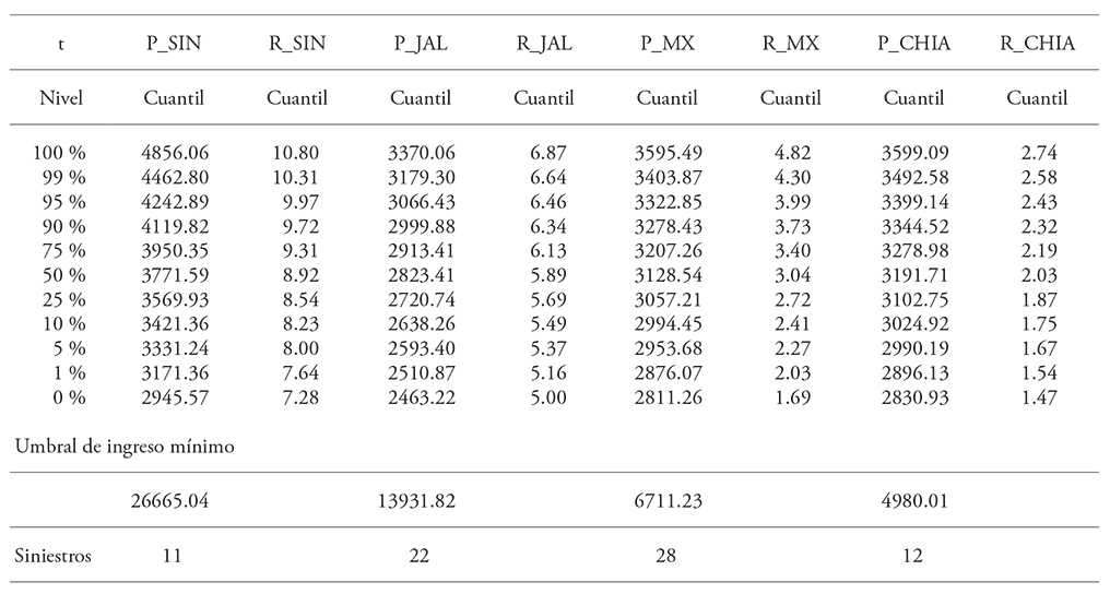
SIN_R: yield in Sinaloa; JAL_R: yield in Jalisco; MX_R: yield in Estado de Mexico; CHIA_R: yield in Chiapas; SIN_P: price in Sinaloa; JAL_P: price in Jalisco; MX_P: price in Estado de Mexico; CHIA_P: price in Chiapas.

An insurance company looking to offer indemnity when income is under a certain threshold might use the estimated quantiles’ results. For instance, when income is under 26 647 in Sinaloa, indemnities have a 5 % probability of occurring in price and yield. However, while considering the 5 % percentile 50 prices and 50 yields below the corresponding threshold would be expected; taken as a whole set the total observations of income per hectare below the threshold is even lower. The total amount of observations under the 26 647 income per hectare threshold are three using the normal copula (Table 3) and eleven using the t copula (Table 4). The amount of claims using each copula differs due to the adjustment to the functions which implies that copula function selection is of relevance (^{Goodwin y Hungerford, 2015}). A comparative study is not presented here; but it is important to remark that if dependencies between prices and yields are not taken into account, the amount of expected claims is higher. This method for risk management, an income policy, would be more efficient. The insurer does not require two policies -one for price and one for yield- which doubles administrative requirements and the risk-averse decision-maker can choose to pay only one premium in a single transaction. Moreover, if the dependencies are exploited the amount of expected claims is lower.

Conclusions

When there are more than one uncertainty sources, risk management can be expensive. Such is the case for price and yield risks; managing them separately would imply double risk premiums, which is compounded if different locations are included. However, if the dependency is modeled, it is possible to build an income risk management instrument that considers price and yield risks simultaneously. This solution may potentially be less expensive both for the insurer and the producer, with a lower amount of claims compared to the separate price and yield policies

REFERENCES

Bekkerman, A., H. Schweitzer, and V. H. Smith. 2014. The impacts of the Canadian wheat board ruling on the North American malt barley markets. Can. J. Agr. Econ. 63: 619-645. [ Links ]
Cleveland, W. S., S. J. Devlin, and E. Grosse. 1988. Regression by Local Fitting. J. Econometrics 37: 87-114. [ Links ]
Goodwin, B. K. 1993. An empirical analysis of the demand for multiple peril crop insurance. Am. J. Agr. Econ. 75: 425-434. [ Links ]
Goodwin, B. K. and A. Hungerford. 2015. Copula-based models of systemic risk in U.S. agriculture: implications for crop insurance and reinsurance contracts. Am. J. Agr. Econ . 97: 879-896. [ Links ]
Goodwin, B. K ., and A. P. Kerr. 1988. Nonparametric estimation of crop yield distributions: implications for rating group-risk crop insurance contracts. Am. J. Agr. Econ . 80: 139-153. [ Links ]
Hennessy, D. A., 1998. The production effects of agricultural income support policies under uncertainty. Am. J. Agr. Econ . 80: 46-57. [ Links ]
Kjersti, A. 2004. Modeling the dependence structure of financial assets: a survey of four copulas. https://www.nr.no/files/samba/bff/SAMBA2204b.pdf [ Links ]
Martínez D., M., y J. García J. 2010. Política de cobertura de precios de maíz en México. Rev. Mex. Econ. Agríc. Rec. Nat. 3: 69-76. [ Links ]
Martínez F., B. 1990. Los precios de garantía en México. Comercio Exterior 40: 938-942. [ Links ]
McNell, A., R. Frey, and P. Embrechts. 2015. Quantitative risk management: concepts, techniques and tools. Princeton (NJ): Princeton University Press. 664 p. [ Links ]
Miranda, M., 1991. Area yield crop insurance reconsidered. Am. J. Agr. Econ . 73: 233-242. [ Links ]
Nelsen, R. B., 2006. An introduction to copulas. New York (NY): Springer Science+Business Media, Inc. 276 p. [ Links ]
Plascencia, T. 2012. Valor en riesgo utilizando cópulas financieras: aplicación al tipo de cambio mexicano (2002-2011). Contabilidad y Negocios 14: 57-68. [ Links ]
Received: June 2016; Accepted: February 2017
Este es un artículo publicado en acceso abierto bajo una licencia Creative Commons