


 nueva página del texto (beta)
 Artículo en XML
 Referencias del artículo
 Enviar artículo por email
 Citado por SciELO
  Similares en
SciELO
Similares en
SciELO 
 Permalink
1. Introduction
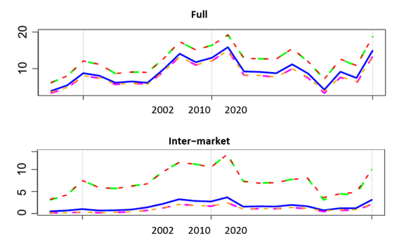
Volatility and correlation increase in global crises such as in the four main crises of the period 2000-2020, namely: the dot.com bubble, the subprime mortgage crisis, the European sovereign debt crisis, and the COVID-19 crisis. The behavior of correlations is the main topic of this paper, so we take the opportunity to provide visual evidence of co-movements in Figure 1. There, a comparison of the main index in the Bolsa Mexicana de Valores (BMV), the IPC index, and the Standard and Poor’s S&P500 index is exhibited. In Figure 2, a comparison for the years 2020-2021 is shown. Volatility is illustrated in Figure 3, where the VIX index is presented. Concerning the afore mentioned episodes of global crises, across-market and across-country correlations are spotlighted and the phenomenon of financial contagion appears. There is a lengthy debate concerning contagion channels and mechanisms, including whether it is a spurious phenomenon generated by a faulty econometric specification; see Forbes & Rigobon (2002). This last point arises precisely because in the turmoil of a crisis, volatility and correlation typically tend to increase simultaneously.
Our goal in this paper is to study how Mexican stocks are interconnected with stocks of the United States (U.S.). To this end, we proceed in two parts. In the first, we estimate partial correlation matrices in every year for the period 2000-2020 and obtain stylized facts. In particular, we obtain a systematic relationship between the two markets. Yet, a subtle rise in interconnectedness is present in the years 2008 and 2020. This provides the motivation to take a closer look for those years which clearly are associated with the subprime mortgage and COVID-19 crises. Hence, in the second part, while we are still interested in how the afore mentioned markets interconnect, we focus on an analysis of those episodes using a zoomed scale which runs a sequence of three-monthly windows.
Our analysis is based on the association of networks to partial correlation matrices and of network centralities. For the estimation of partial correlation matrices, we follow the statistical procedure explained in subsection 2.4 below. It is an implementation of the estimator in Meinshausen & Bühlmann (2006) of neighborhood selection in a sparse high dimensional graph.
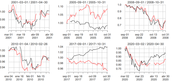
Note: The red line is the IPC index while the black line is the S&P500 index. For critical years, a notable convergence of time series appears while for the relatively “tranquil” years 2005 and 2017, indices diverge.
Figure 1 Comparison of (normalized) S&P500 and IPC indices.
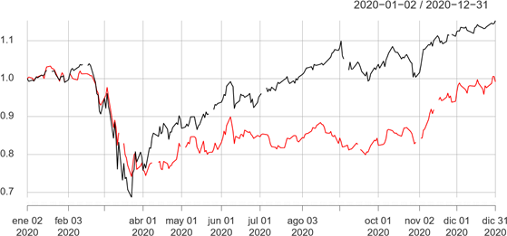
Figure 2 Comparison of (normalized) S&P500 and IPC indices during the current COVID-19 pandemic. Co-movements are evident.
In an early stage of the empirical research we also experimented with more traditional multivariate versions of time series models in order to estimate correlation matrices. However, they were unfeasible due to numerical instabilities from data dimension. The estimated partial correlation matrices are then interpreted as adjacency matrices of a graph from which centralities are estimated.
To the best of our knowledge, analysis of stock market linkages between the U.S. and Mexico based on partial correlations estimated with the statistical procedure that we apply here is new. Beside its novelty, we chose this approach for its ability to handle data over small time intervals, since it solves the trade-off between data size and statistical accuracy.
Most studies focus on aggregated data analysis at the level of market indices, particularly so for the Mexican stock market. Our approach is based on network theory and we study here at the level of individual stocks to achieve more granularity. A distinguishing element in the paper is the association of a network to a correlation matrix. This interpretation has the convenience of an agile visualization while allowing for the application of network metrics. We compute degree and eigen centralities metrics which allow the consolidation and quantification of a full picture of network dynamics. In particular, this method does not apply if we only focus on indices, since in our case this means considering the data of two time series. In order to have a reference for a comparison, we also report some results based on Pearson correlations. Our estimations record a stability for partial correlation matrices not present for Pearson correlations. Indeed, the time series of centralities move in a small bandwidth of around 20 percent for partial correlation matrices for the period 2000-2020. In contrast, centralities for Pearson correlation matrices require a bandwidth of more than 300 percent. More on this in Section 3.1.
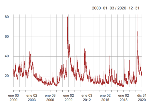
Note: Local maxima visualized as peaks are located around the turmoil of the crises. The VIX level during the period of the COVID-19 pandemic is of the same magnitude as for the subprime mortgage crisis.
Figure 3 Visualization of the VIX index during the different critical years of the period.
After this introduction the paper is organized as follows. In Section 2 we expand this introduction and provide preliminaries for our analysis. More specifically, in subsection 2.1 we discuss the topic of stock return co-movements and in subsection 2.2 relate this discussion to the specialized literature. In subsection 2.3 we review literature on the relevance of sector classification with respect to price movements, since one of our main findings appears at this level. In subsection 2.4 we provide methodological details in the estimator of partial correlation matrices. In subsection 2.5 we briefly present the concepts of eigen and degree centralities. In subsection 2.6 we furnish details of the input data for our estimations. In subsection 2.7 we explain the taxonomy of stocks by sector.
In Section 3 we report our findings based on the estimation of partial correlations for each year for the period 20002020 and discuss their financial implications. In Section 4 we focus on the subprime and COVID-19 crises and report the results of estimation and their financial interpretation. Section 5 concludes with a final discussion elaborating on the main findings of the paper.
2. Material and Methods
In subsection 2.1 below we discuss the co-movement of stock prices, in general and particularly between Mexico and the U.S., and then in subsection 2.2 we relate this discussion to selected papers from the specialized literature. In subsection 2.3 we review literature concerning sector interconnectedness. The other subsections provide information concerning methodology, data and its processing.
2.1. Co-movements of stock returns
Correlation and volatility are related, and this relationship is an empirical fact extensively discussed in the literature. In the turmoil of a crisis, stock prices have the usual characteristic of generating more correlation and exhibiting slumps. This is a specific pattern of co-movement and is the temporal characteristic in the definition of bear markets.
Particularly unique is the case of North America with strong trade ties, which, notwithstanding benefits, many studies find to be a transmission channel of financial contagion. Especially between important trade partners U.S. and Mexico some papers find that economic recession and financial distress originating in the U.S. during the subprime mortgage crisis was transmitted to Mexico, mainly due to a slowdown in trade that also impacted on financial markets. We do not directly investigate here if financial contagion is present, when, and how, since this is a problem that has its own methods, the literature is extensive, and our objective is distinct. Instead of implementing methods commonly used in the field of financial contagion, we focus on the method of network centralities which provide a useful description that will account for an insightful element of analysis and provide information about price co-movements. Thus, in the context of price co-movement, quantified by correlation, we formulate the following questions which accompany the main goal of the paper:
Does the BMV equity market have a permanent relationship with stocks traded in the U.S.? What is the dynamic of this relationship through the years?, particularly, how is the relationship in the years of crises?, and to what extent quantitative metrics are able to distinguish between the different crises?
To answer these questions, we compute correlation matrices for stocks in the BMV and stock components of the S&P500. We decided to study correlations instead of covariance since the former is widely used in the study of price co-movements, while the latter is more common in portfolio allocation theories. The use of partial correlations is motivated in order to mitigate the record of indirect relationships between stocks. This is particularly relevant for our study since endogenous activity in the market impacts some fundamental quantities such as volatility and correlation. There is also an effect between stocks due to trading and our results suggest that partial and Pearson correlations behave differently in this sense. Indeed, comparisons that we include in the paper clarify this point.
On pursuing our goals we follow an approach based on network theory and study networks based on correlations of stocks between Mexico and the U.S. within a common framework. In the literature a significant number of papers agree on the fact that correlations are dynamic and change with respect to time. Hence, as already formulated in our main questions, an important aspect of the present study is about the time evolution of the financial network of stock markets with emphasis on the crisis episodes for the period 2000-2020.
We focus on stocks traded on the BMV (not restricted to the components of the main IPC index) and stock components in the S&P500 index. We analyze at the level of stocks and do not include indices. Therefore, we gather together time series of log-returns for stocks in the BMV and stocks forming the S&P500 index and estimate correlation matrices. In order to establish and describe stylized facts, we estimate one matrix for each year for the period 2000-2020. The off-diagonal components of those matrices are interpreted as adjacency matrices of a weighted graph. There is a new stock market in Mexico called the Bolsa Institucional de Valores (BIVA) which started operations in 2018. Thus, it is quite recent for the purposes of this study. As for the stock market in the U.S. we focus on the components of the S&P500 index since these stocks are considered to be representative of the American stock exchange and are diversified across industrial sectors.
In Figure 1 a comparison of the S&P500 and IPC indices is illustrated. At this level of aggregation, the time series of the IPC and the S&P500 indices present certain co-movement during the main crises over the period 2000-2020, while on the central graphs for the years 2005 and 2017 a certain level of divergence can be appreciated. In Figure 2 we present the complete year for 2020 and January-2021. Again, at this point based only on the visual evidence, the co-movement of both indices is evident, particularly so in the severe drop in March 2020, with a generalized lockdown provoking a sudden and severe economic break across the globe, caused by governmental response to the COVID-19 pandemic. Financial markets reacted as can be appreciated from the severe slump in index values and the tremendous peak of volatility. In this case, co-movement seemed to be the consequence of a combination of the pandemic and the halting of the economy. As a matter of fact, in difficult years we see that the IPC index behaves like the S&P500 index. However, the nature of the crises is different, specially their origins. In the subprime crisis the consensus is of financial contagion, while in the COVID-19 pandemic, opinion points to origins outside financial markets; see Rodríguez-Benavides, Gurrola-Ríos, & López-Herrera (2021), Hanif, Mensi, & Vo (2021). Hence, in order to reconcile the anecdotal evidence with the quantitative metrics, it would appear to be essential to find contrasts at different levels of granularity. This comparison motivates our study, and we estimate correlations at the scale of individual stocks. At disaggregated scales various phenomena appear, Bekaert & Wu (2015) document volatility asymmetry due to covariance asymmetry at the firm level. In the case of Mexico there are heterogeneous reactions at the level of geographical disaggregation; see e.g., Jaramillo-Olivares & Jaramillo-Jaramillo (2016). In our study, disaggregated data at the firm level allows us to analyze interconnections by industrial sector, which proves to be very useful. Moreover, we will see that estimated centralities shows a faster reaction to main events in comparison to simply computing Pearson correlations from indices.
2.2. Literature on co-movements
Dooley & Hutchison (2009) study how financial markets in a selection of emerging countries reacted to news generated in the U.S. in the period 2007-2009 around the subprime mortgage crisis. The main input is based on Credit Default Swaps (CDS). They find decoupled emerging markets from early 2007 to 15 September 2008 (“The Lehman Brothers Day”). However, after this date, emerging markets, including Mexico, became more receptive to the situation in the U.S. financial system. Differentiated responses at different lapses in time asserts convergence-decoupling as a dynamic phenomenon. Quite intriguing, despite very limited subprime exposure, the Lehman Brothers bankruptcy announcement fostered greater links in equity markets between Mexico and the U.S. During the subprime crisis Mexico experimented an increase in volatility and asymmetry (Sosa, Ortiz, & Cabello, 2017) and intra-market correlations magnified in Mexico; see Trevino Aguilar (2020).
From Dooley & Hutchison (2009)’s approach based on “regression event study” one could argue about the key role of information in the process of transmission. However, the impact of news cannot be generalized to systematically having an impact in all situations or for all kinds of information. Indeed, Roll (1984), Cutler, Poterba, & Summers (1989) and Campbell & Kyle (1993) find that a large share of intramarket price co-movements cannot be attributed to news items. There are studies in which news items do not alter correlations across countries. Karolyi & Stulz (1996) investigate daily, and intra-day return co-movements between Japanese and U.S. stocks. They observe a diminished reaction in across-market covariances with respect to macroeconomic announcements. They also find that correlation is high when markets are volatile. Typically, bear markets are volatile and Longin & Solnik (2001) find that correlation increases in bear markets for equity markets in the United States, the United Kingdom, France, Germany, and Japan for the period January 1959 to December 1996.
Forbes & Chinn (2004) find that trade is the most important determinant of how the world’s largest markets affect financial markets around the globe. Particularly between the U.S. market, probably the world’s largest, and the BMV, a much smaller one. Forbes & Chinn (2004) also find that bilateral foreign investment is much less relevant. Johnson & Soenen (2003) find that for Mexico (and other countries in the region) the high level of trade with the U.S. has a strong positive effect on stock market co-movements. Lahrech & Sylwester (2011) find an accelerated integration process of Mexico with the U.S. within the period of the North American Free Trade Agreement (NAFTA). The impact of NAFTA in the equity markets is studied in Lahrech & Sylwester (2013).
This integration process extends to the synchronization between financial and business cycles across countries. Concerning business cycles, Mejía Reyes, P. and Campos, J. (2011) find synchronization between Mexican manufacturing production and the U.S. business cycle. However, it is heterogeneous at the level of states. Possible reasons can be attributed to disparities in foreign direct investment; see Mejía-Reyes, Rendón-Rojas, Vergara-González, & Aroca (2018). Roman de la Sancha, Hernandez Alvarez, & Rodriguez Garcia (2019) find synchronization between financial cycles in the period 1991-2018 for the Dow Jones and the IPC indices, which is supported for the Americas region by evidence from Rodriguez-Nieto & Mollick (2021) for the period 2002 to 2015, and also by Sosa & Ortiz (2017) for the NAFTA countries between 2003 and 2015, while Reyes-Zarate, F. J. and Ortiz, E. (2013), report a relatively stable period from 2003 to 2007 just before the subprime crisis and conclude that regional diversification of stock holdings is still essential due to varying degrees of development and stability in the three NAFTA markets. López-Herrera, F. L. and Santillán-Salgado, R. J. and Cruz-Ake, S. (2015) come to the same conclusion in their study of the Mexican stock market and a World stock market index between 1987 and 2012. Cruz-Aké, S. and Ramírez-Alatriste, F. and García-Ruíz, R. S. (2012) use Chaos Theory to report significant phase synchronization between international stock markets in the period 2003 to 2012 for a selection of international stock markets which includes Brazil but excludes Mexico and suggests reduced earnings for stock diversification. Integration not just in the NAFTA countries but also in the Americas as a whole appears to be the trend as Lopez Villa & Sosa Castro (2021) report in a study of the capital and currency markets of México and Brazil between 2000 and 2020.
After the subprime mortgage crisis, the next global episode was the European sovereign debt crisis and Kalbaska & Gatkowski (2012) feature the role of the former crisis in stirring up the European debt crisis. Based on CDS data, the authors find “several waves of contagion defined in terms of an increase in conditional correlations”. Alter & Beyer (2014) determine spillover effects during the European sovereign debt crisis with periods of intense contagion around policy events. They also find an increase of the interdependency among banks in the Eurozone. In the case of Mexico, the debt crisis had an impact, and among other routes, the banking sector was arguably a transmission channel of distress due to liquidity constraints of foreign banks with operations in the country; see Toledo-Patiño (2012).
An increment of volatility in stock returns can be the consequence of exogenous news or endogenous activity in the market. Concerning the distinction in the origin of increased volatility, Sornette, Malevergne, & Muzy (2003) note that the volatility drop in the American stock exchange after the October 1987 crash is described by a power characterize the former episode as endogenous while the second as exogenous. Thus, following a volatility shock the law Δ𝑡 −0.3 while volatility after the September 11 attack decays according to the power law Δ𝑡 −0.5 . Moreover, they recovery speed depends on the origin of the episode. Elaborating on the idea that an increase in volatility can be in its origin endogenously generated by trade activity, Ben-David, Franzoni, & Moussawi (2018) find evidence that the increase in stock return volatility is likely a reflection of the transmission of non-fundamental demand shocks from the ETF market to the prices of the underlying stocks via trading activity. They find that activity between ETFs and their baskets magnify the effect on volatility. Trading activity as a mechanism of financial contagion in a specific context is documented by Boyer, Kumagai, & Yuan (2006). In their discussion international traders play a major role.
2.3. Literature on sector intra-connectivity
Early studies of stock markets open the debate as to whether stock markets move on a country or economic sector basis. Livingston (1977) studying the New York Stock Exchange found that up to 26% of the volatility of equity shares could be explained by industry factors. Roll (1992) found that in advanced markets, industry concentrations were a significant factor in explaining global stock price behavior. Baca, Garbe, & Weiss (2000) ascertain that historically, country effects have been dominant in explaining variations in global stock returns, even in the developed markets, and investors have segmented their allocations accordingly. However, there has more recently been a significant shift in the relative importance of economic influences, and in developed markets, the impact of industrial sector effects is now roughly equal to that of country effects. Cavaglia, Brightman, & Aked (2000) using developed country data, conclude that diversification across industries provides greater risk reduction benefits than diversification across countries. Kearney & Poti (2006) conclude that non-country factors drive the volatility of equity returns and in particular industry-based strategies might outperform country-based diversification strategies. They focus on the advanced markets of France, Germany, Italy, Netherlands and Spain for the period 1993 to 2002.
Shen & Zheng (2009) study the Chinese market and report that the interactions between stocks within business sectors are weak. In the case of China, the strength of intra-sector stock market correlations appear to be weaker than in the U.S. market and other, older European markets, and in India, economic sector correlation is weaker still. Other emerging markets show similar behavior, i.e., that country effects are stronger than sector effects. Jung, Chae, Yang, & Moon (2006) using MST network techniques, find that the Korean stock market, at the time an emerging market with a small number of very large conglomerates and a much smaller number of total companies than is the case with the U.S., does not correlate by sector. As we will demonstrate in this paper, this agrees with the experience of Mexico in which intra-sectoral correlations are weak in comparison with sectors in the U.S.
2.4. The estimation of partial correlations
In this section we explain in more detail the underlying model that we are going
to estimate for the partial correlation matrices. Let
Now, we define an adjacency matrix 𝐏=(Pi,j) which will be our definite input for the network based on partial correlations. It is defined by
In order to obtain the partial correlation coefficients, we do not estimate
where n represents the number of stocks, 𝜃 determines the distribution’s
expected value, 𝐴(⋅) is a normalizing constant and the set of parameters
2.5. Centralities
Centrality in graph theory assesses how influential a vertex is immersed in its
graph. There are local and global metrics. In our financial application, for the
local metric of degree-centrality, the intuition is that an
influential stock in the financial network relates to the behavior of a large
number of vertexes in the network. For a given vertex in a weighted network, its
degree-centrality is the weights’ sum of connecting edges. The second measure of
centrality that we estimate is the eigen-centrality and it is a
global metric. The estimation of eigen-centralities transfers to a spectral
analysis of the adjacency matrix associated with the graph. Let us explain in
more detail how it is defined. Let
Thus, the vector
2.6. Data
As our main input we use time series from Yahoo Finance. We gather together in a unique database, times series from BMV stocks and components in the construction of the S&P500 index. We focus on daily closing prices. The complete list of analyzed stocks can be found as supplementary material. The frequency of data is daily for a period of time starting in January-2000 and ending in December-2020. For the first part we organized data in windows of one year (from January to December) in which a filtering process is applied in two steps. In the first step, for each year, stocks in the market with the most complete information were selected. The criterion was that only stocks with more than 90% of all the available dates are selectable. Then, in a second step, stock prices not having a minimum of variance in moving windows spanning 30 observations were discarded. For the second part in which we concentrate on the subprime and COVID-19 crises, we consider a moving window of non-anticipative 60 observations which approximately spans three months. The same filtering process is applied for the years 2007-2008 and 2019-2020.
Correlation matrices are estimated from log-returns:
2.7. Configuration of industrial sectors
Standard Industrial Classification (SIC) codes is the classic system in the U.S. although the similar North American Industry Classification System (NAIC) is now used in the U.S., Canada, and Mexico. However, a generalized use of this last system is still far from being standard. For this reason, we show how stocks are grouped by industry sector in the BMV and S&P500 classifications.
For stocks in the BMV, sectors are listed in Table 1 and for stocks in the S&P500 index, in Table 2. Figure 4 presents an estimated network in which stocks can be identified in their sector.
3. Partial correlations
3.1 Stylized facts
In this section we report the results of estimating partial correlation matrices. We estimate a partial correlation matrix and the adjacency matrix 𝐏 for each year in the period 2000-2020 using the specification (2). A graphical representation of partial correlations is displayed in Figures 5 and 6. In Figure 5 only inter-market edges are presented with edges joining a stock in the S&P500 Index and a stock in the BMV market. In Figure 6 only intra-market edges are presented with edges joining a stock in the S&P500 index with another stock in the S&P500 index (respectively a BMV-stock with a BMV-stock).
Table 1 Industrial sectors in the BMV
| Sector | No. Stocks | Description |
|---|---|---|
| 1 Basic consumption | 21 | Manufacturers and distributors, food, and beverage companies |
| 2 Energy | 2 | Energy producers, equipment, services, and distribution |
| 3 Financial services | 25 | Includes banks, financial and insurance firms |
| 4 Health | 4 | Care providers, equipment, supplies and pharmaceuticals |
| 5 Industry | 36 | Includes companies providing equipment and services in the production chain |
| 6 Information Technology | 1 | Software and Hardware for information technologies |
| 7 Materials | 22 | Includes companies providing input materials in the production chain |
| 8 Non-basic consumption | 19 | Includes retailers, consumer service providers and consumer durables |
| 9 Telecommunications | 9 | Includes wireless providers, internet service providers and satellite companies |
Table 2 Industrial sectors for stocks in the S&P500 index
| Sector | No. Stocks | Description |
|---|---|---|
| 1 Communication Services | 26 | Wireless and internet service providers. Satellite companies |
| 2 Consumer Discretionary | 61 | Automobiles (industry and distributors), Hotels & Restaurants, Household durables. |
| 3 Consumer Staples | 33 | Beverages Industry, Food Products, Personal Products. |
| 4 Energy | 26 | Equipment & Services, Oil, Gas & Consumable Fuels. |
| 5 Financials | 66 | Banking, Capital Markets, Consumer Finance, Insurance, Mortgage Real Property. |
| 6 Health Care | 62 | Biotechnology, Equipment & Supplies Industry, Pharmaceuticals. |
| 7 Industrials | 73 | Aerospace & Defense Industry, Air Freight & Logistics Industry, Airlines, Building Products. |
| 8 Information Technology | 70 | Communications, Electronic Equipment, Instruments & Components, IT Services. |
| 9 Materials | 28 | Chemicals, Construction Materials, Containers & Packaging, Metals & Mining. |
| 10 Real Estate | 31 | Equity Real Estate Investment Trusts, etc. |
| 11 Technology | 1 | Tyler Technologies. |
| 12 Utilities | 28 | Electric Utilities Industry, Gas Utilities, Independent Power and Renewable Electricity Producers. |
Note however that for each year both figures are based on a common estimation of partial correlation matrices. We only include graphs for the years 2000 to 2019, due to space constraints, but see Figure 7 for inter-market connections in the year 2020. The graph of partial correlations for that year is quite similar to other years and its network centralities are studied in sections below.
We obtain the following stylized facts from the correlation-based graphs:
From partial correlations, Figure 5 evidences a systematic relationship of the BMV with the U.S. stock market. Staying with the visual evidence, it is hard to appreciate any dramatic change in the network topology across the years. This is an observation that will be confirmed through the estimation of network metrics, the degree and eigen-centralities; see the panels of Fig. 8 below. For a quantitative assessment, eigen-centrality in the top panel of Fig. 8 moves in a bandwidth of around 20 percent with respect to its minimum eigen-centrality value of 0.7 units.
Estimations of centralities based on Pearson correlations are illustrated in Figure 9. Centralities clearly present higher levels in the years of crisis. Hence, they are monotone with respect to volatility. Eigen-centrality in the top panel of Fig. 9 moves in a bandwidth of more than 300 percent with respect to its minimum eigen-centrality value of circa 38.5 units.
Figure 6 shows that several sectors in the U.S. market exhibit many intra-sector links (stocks in the same sector are connected). This is a systematic phenomenon across the years of the period. In contrast, for the BMV there are few links between stocks in the same sector. This is illustrated more clearly for the year 2020 in Figure 7, left-hand side. Actually, there is a certain level of robustness in this property. Indeed, the right-hand side of Figure 7 shows a network based on Pearson correlations. This graph reveals the same phenomenon of high contrast in terms of intra-sectorial links for S&P500 and the BMV.
Beyond visual evidence, network centralities by sector quantifies this contrast; see Figures 10 and 11 below.
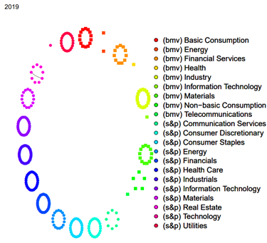
Note: Stocks from the S&P500 index are represented by circles. A node representing a stock from the BMV market has a square shape. As visual guide, the BMV sectors start clockwise at 12:00 and then advance to the right up to circa 5:00.
Figure 4 An example of how stocks are organized by sectors in the associated networks.
3.2 Estimated centralities
In Figure 8 below we see estimated centralities for our networks. The blue line is the per-year eigen-centrality of the network (determined as the largest eigenvalue of the adjacency matrix) and delivers a global metric for the complete network. The green line is the maximum degree-centrality by year. The red line is the maximum of degree-centralities’ absolute values. Thus, for the red line we first computed the absolute value of every component of the matrix P, then the sum of weights for each column, and finally the maximum. The pink line is the average of degree-centrality and in orange the average of absolute degree-centrality. Hence, for the orange line, as for the red line, we first computed the absolute value of the matrix 𝐏.
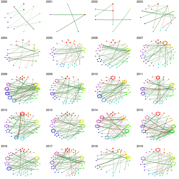
Note: Only inter-market edges are presented with edges joining a stock in the S&P500 Index and a stock in the BMV market. As a visual guide, BMV sectors start clockwise at 12:00 and then advance to the right up to circa 5:00.
Figure 5 Graphs based on partial correlation matrices, by year, in the period 2000-2019.
In the top panel of Figure 8, we see time series of centralities for the graphs based on partial correlations. Although there are some small variations, the lines are stable across the years in that they move in a small bandwidth. The distance between the lines presenting averages (pink and orange) and the lines presenting maximums (green and red) indicate a distribution in signs and that there are positive and negative correlations. We do not include the graph for the network of intra-connections in which only stocks in the same market are connected since its almost identical to the full network. Hence, for our data, intra-market links dominate in the estimation of centralities, but inter-market links tell their own story. Indeed, there is an interesting story coming up next.
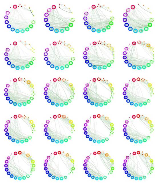
Note: Only intra-market edges are presented with S&P500-to-S&P500 stock links (respectively BMV-to-BMV stock links). Again, BMV stocks start clockwise at 12:00 and advance clockwise to 5:00.
Figure 6 Graphs associated with partial correlation matrices, by year, in the period 2000-2019.
In the bottom panel of Figure 8, only across-market edges connecting BMV-stocks to S&P500-stocks are included in order to estimate centralities. These centralities unravel interesting information. In contrast with the top panel, here time series present a more dynamic structure. Significant difference between the red and green lines in the year 2008 appear. They represent maximum of degrees, which in the case of the red line is the maximum of absolute values. This difference indicates the appearance of negative partial correlations. Relative to 2008 the five stocks with the highest degree calculated from absolute values are ICA, ARA, GMEXICO, IDEALB-1, CEMEXCPO and GFNORTEO. All except for CEMEXCPO have differences concerning their degrees (no absolute values) suggesting a balance for those stocks between positive and negative correlations. It is remarkable the industry sector to which these stocks belong to, and more specifically their activities are closely related to the construction industry (ICA, ARA, CEMEXCPO) and financial services (GFNORTEO).
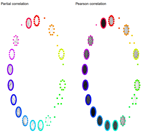
Note: Only edges connecting stocks in the same market and the same sector are illustrated. For comparison, on the left-hand side the graph of partial correlations is presented and on the right-hand side the graph of Pearson correlations. On both networks, industrial sectors in the U.S. are more interconnected than in Mexico.
Figure 7 Graphs for the year 2020.
As seen from the sign of partial correlations, it is worth mentioning that despite the high severity of the subprime crisis, there are negative correlations. Relationships divide into procyclical and countercyclical movements with respect to the U.S. market represented by the components of the S&P500 index. This division is also observed for the European sovereign debt crisis. Thus, indicating a taxonomy of how stocks react over critical periods.
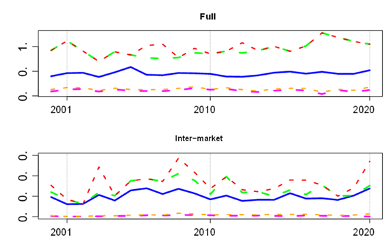
Note: The blue line is the time series of network eigen-centrality. The green line is the maximum degree-centrality by year. The red line is the maximum of degree-centralities’ absolute values. The pink line is the average of degree-centrality and in orange the average of absolute degree-centrality. On the top panel centralities are computed from the full graph. On the bottom panel centralities are computed considering only across-country edges.
Figure 8 Network centralities from partial correlation matrices.
For comparison, we illustrate in Figure 9 centralities based on Pearson correlations. The contrast is clear, the level of magnitude from Pearson correlations is far too high, the peaks of centralities are clearly associated with the main crises in the period and the effect is so strong that all the illustrated curves present identical structures. These metrics clearly point to an increase in correlation and determine a less stable network topology in comparison with partial correlations. However, considering this is a signal of a closer association between stocks, it should be taken at face value. As Figure 3 illustrates, increments in volatility synchronize with crises and this might be the explanation of higher (Pearson) correlation in the metrics; this is the main point in Forbes & Rigobon (2002).
Note: The colors have the same meaning as in Figure 8. The top panel presents centralities for the complete network with correlations from the ordering of stocks in the S&P500 and the BMV. The bottom panel side presents centralities for the restricted network of links connecting stocks across countries.
Figure 9 Network centralities from Pearson correlation matrices.
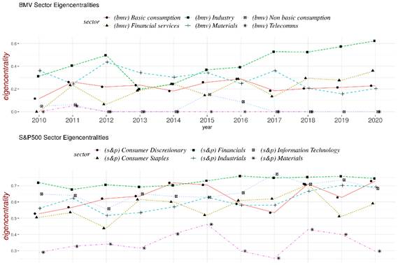
3.3 Sectors
In Figure 10 we present time series of eigen-centralities estimated by year and by industrial sector from networks based on partial correlations. In the upper panel the information is for Mexico and in the lower panel the corresponding information is for the U.S. The reader should compare the y-axis to confirm that the eigen-centralities for the Mexican market are lower than those for the American market. In Figure 11 an analogous comparison is presented with respect to mean degree-centralities and the same conclusion holds true. Thus, confirming through network metrics the visual evidence of low connectivity of sectors in the BMV, Figure 7, left-hand side.
In Figure 10 we observe that the eigen-centralities in the years 2019 and 2020 for the BMV Industry sector throws up levels comparable to those in the S&P500. Hence, it is worth taking a closer look at the partial correlation matrices for this sector and those years. The matrices are sparse with most of the entries equal to zero. In Table 3 below we report the links with partial correlations above the threshold 0.1. The tickers ASUR, GAP and OMA listed in the table identify firms with transportation activities, more specifically they control main airport systems in Mexico. The tickers PINFRA, GICSA and VESTA identify companies dedicated to infrastructure construction. This quantitative result in the metrics seems to be the expression capturing a key conjuncture in the country about a public investment project for the construction of a new airport. In fact, there is a major project to update the Benito Juarez airport, which is the main international hub of the country. Hence, there is a tangible factor from the real economy that the market priced in this period for this family of stocks. In this sense, partial correlations capture an increase in co-movements attached.
Note: Networks based on partial correlations.
Figure 10 Eigencentralities by sectors in the period 2000-2020.
Table 3 Most significative partial correlations in the Industry sector for the years 2019 and 2020.
| tick1 | tick2 | weight | year | tick1 | tick2 | weight | year |
|---|---|---|---|---|---|---|---|
| ASUR | GAP | 0.3 | 2019 | ASUR | OMA | 0.15 | 2019 |
| GAP | OMA | 0.3 | 2019 | GAP | PINFRA | 0.1 | 2019 |
| GICSA | VESTA | 0.1 | 2019 | ||||
| ASUR | GAP | 0.4 | 2020 | ASUR | OMA | 0.2 | 2020 |
| GAP | OMA | 0.4 | 2020 | ||||
To a change in the stocks’ fundamentals. Moreover, in Figure 11 we see means of degree centralities. Here, nothing spectacular happens for the BMV sectors and in particular the BMV Industry sector does not separate from the others. This makes perfect sense since the partial correlation matrices are sparse.
4. Similitude and contrast in the subprime mortgage and COVID-19 pandemic crises
In this section we compare network metrics in periods englobing the subprime mortgage crisis and COVID-19 pandemic. We start by providing some information concerning the latter period and refer to the relevant literature for the background on the subprime mortgage crisis.
4.1 Key takeaways from the COVID-19 pandemic
In the year 2020 the COVID-19 pandemic shook the world. Starting as a located outbreak, it soon scaled into a pandemic and affected many aspects of humanity. There are clear impacts in the real economy and the well-being of families. Financial systems have also internalized the crisis and as we will show, across-country linkages changed as a result. In the analysis of the next subsection the month March-2020 marks different qualitative properties of network centralities time series. But before considering financial aspects, March-2020 represents an inflection point during the development of the pandemic.
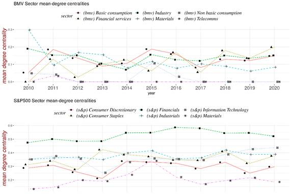
Note: Networks based on partial correlations.
Figure 11 Mean degree centralities by sectors in the period 2000-2020.
On March-2020 the world witnessed the start of a global response against the COVID-19 pandemic with a variety of public policies, most notably a generalized “lockdown”. To substantiate the qualifier “globalized”, in Figure 12 we present the Oxford stringency index for the following selection of countries: Austria, Brazil, Canada, Czech Republic, Finland, France, Germany, Japan, Luxembourg, Netherlands, Portugal, Romania, Slovak Republic, Spain, Sweden, the U.S. and Mexico. The highest levels of the index represent stricter responses to the pandemic. It is clear from the Oxford stringency index that all the countries in the list started strict security initiatives in March-2020. Those measures included the lockdown of cities and regions, which ultimately led to a sudden economic halt as can be inferred from Figure 13 below. Figure 13 below presents the Production index for the following list of countries: Austria, Brazil, Canada, Czech Republic, Finland, France, Germany, Japan, Luxembourg, Netherlands, Portugal, Romania, Slovak Republic, Spain, Sweden, and the U.S. The time series were downloaded from the corresponding Government agencies but our starting point was a directory of the International Monetary Fund. Again, March-2020 represents the turning point when the index started to sink with local minima around April or May.
4.2 Comparison of centralities
We have seen in the time series of Figures 8 and 9 that complementary stories are told by centralities based on Pearson and partial correlations for the complete network and for the subnetworks of across-market linkages. Strongly marked local maxima for time series are obtained from Pearson correlations while partial correlations reacted smoothly with respect to these crises. As indicated previously, the evidence suggests that Pearson correlations are conditional on volatility, and so it is possible that centralities inherit this condition. On the other hand, centralities based on partial correlation matrices are less sensible with respect to this condition. A closer look to Figure 8, bottom panel, exhibits a mild upwards trend in 2008 for the red line (maxima of absolute value) and in 2020 for the red and blue lines (maxima of absolute value, and eigen-centrality, respectively). Hence, we look in more detail into time series for these specific years.
In Figure 14 we report inter-market centralities based on partial correlations estimated from a sliding window. Each window is computed daily and accounts for approximately a span of three months.
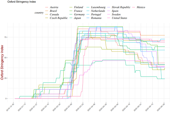
Source: Authors’ own elaboration with Oxford University data.
Figure 12 Oxford Stringency index for a selection of countries.
Recall that in a month there are circa 20 activity days in which markets are open. On a day with an index 𝑥 we consider the window starting with the observation 𝑥 − 60 and ending on 𝑥. Hence, the metrics are reported in a non-anticipative way in the sense that for each day only data from previous days has been used.
In fact, the estimated time series exhibit an interesting feature. In the left-hand panel of Figure 14, the metrics for the second semester of 2008 are shown. Clearly this is a period related to the subprime mortgage crisis and in particular during September came the announcement of the Lehman Brothers bankruptcy. Beyond the up-and-down swings it can be appreciated that between July and August of 2008 the centralities soared relative to values on other days. An analogous description follows for the right-hand panel presenting the metrics for the first semester of 2020, obviously related to the COVID-19 pandemic. Between February and March, we see centrality metrics with high levels relative to other days.
Thus, degree and eigen centralities are telling similar stories for turbulent periods of time with quite different backgrounds. But what is this similitude? First of all let us recall that partial correlations provide direct relationships reducing the possibility of associating two stocks that are related through a third one. So, it suggests that for both episodes there was an increase in direct relationships previous to big events (the announcement of the Lehman Brothers bankruptcy and the launch of the lockdown, respectively). Now, let us distinguish between noisy and informed trading in the tradition of Black (1986). The information attached to direct connections suggests that investors trade on their information to internalize pessimistic expectations in fundamental values. Now, we are not saying that an investor holds an international portfolio with stocks from both markets (which nevertheless is possible). But we are saying that there is mutual information for investors with holdings in the U.S., respectively Mexico, markets leading their actions and producing co-movements, at least for some stocks. To support this claim about mutual information, recall that previous to Lehman Brothers bankruptcy there was already tremendous agitation with respect to important losses produced by mortgage-backed securities (MBS). More precisely, by 2007 Bear Stearns hedge funds on MBS had already incurred billionaire losses and on March-2008 the Federal Reserve facilitated a 25 billion loan to provide liquidity, yet the company entered into bankruptcy. Moreover, Lehman Brothers company had reported spectacular losses before, but close to, September-2008. Specifically, by June-2008 the company reported losses of not less than 2.8 billion USD and the company stock shrank to 73% of its value.
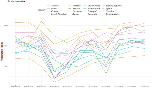
Source: Authors’ own elaboration with time series downloaded from the corresponding Government agencies.
Figure 13 Production Index 2020.
Thus, the environment in financial markets, specially related to MBS, carried bad news of accrued losses by large firms. Note that June-2008 is included in the period that produced higher levels of centrality in Figure 14. Let’s now move forward in time and discuss the COVID-19 pandemic. To this end, we first start with a brief recount of key events. The coronavirus disease was first identified in Wuhan China in December 2019. The World Health Organization declared the outbreak an emergency of international concern in January-2020 and a pandemic in March-2020. In January-2020 the situation in European countries captured international attention since the virus was spreading very fast there. Thus, again, we identify from December-2019 to January-2020 days with bad news reporting a bad situation. Although at that time the magnitude of the pandemic and its consequences most probably were unpredictable, a reasonable guess is that investors already had pessimistic expectations.
Thus, we claim that the similitude on both sides of Figure 14 is due to information being internalized in the equity markets. Information about the real economy that would impact the fundamental values of assets.
We present centralities based on Pearson correlation matrices in Figure 15 below.
Let us start with an evident comparison. There is a huge increase of degree centrality on the right-hand side, which seems to signal a jump, and a large one. On the left-hand side, we also see an increasing tendency but not so steep. This makes sense. For the subprime mortgage crisis, the year 2007 was already turbulent with a contained but unusually high volatility. This comes in tandem with maintained high correlation levels across-markets for 2007 and the first semester of 2008. Then, as the second semester of 2008 advanced, volatility and correlation also increased. Apparently, this was the “market prediction” of a forthcoming big event. Of course, the exact event was unknown, particularly nobody could forecast the Lehman Brothers bankruptcy with certainty. Now let us take a look at the other crisis. Starting from the outbreak in Wuhan China, the development of the pandemic was very fast. Already in January-2020 there was big media coverage of the contagion in Europe, particularly in Italy and then Spain. Perhaps it is not an exaggeration to say that, beyond the financial world, it was the start of an anticipated recession transforming every aspect of society. In particular, it caused the reaction of financial markets all over the world. Indeed, this accelerated development, full of bad news, formed pessimistic expectations leading to an increase of volatility and correlation.
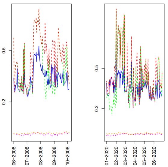
Note: Matrices are computed daily in a non-anticipative running window of 60 observations. The left-hand side panel reports around September-2008 when the Lehman Brothers bankruptcy was announced. The right-hand side panel reports around March-2020 when lockdowns around the world were launched as a global response to the COVID-19 pandemic.
Figure 14 Network centralities based on partial correlations.
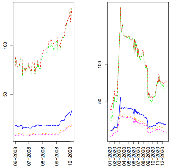
Note: Matrices are computed daily in a non-anticipative running window of 60 observations.
Figure 15 Network centralities based on Pearson correlations.
To conclude this section, we include in Figure 16 the graph of Pearson correlations for the S&P500 and IPC indices for the subprime mortgage crisis. Correlations are estimated from a sliding window of 60 observations. It is clear that the time series “rallies-up” after September 2008. Thus, it reacts after the main event of the Lehman Brothers bankruptcy announcement, in contrast to centralities that react circa three months before.

5. Conclusion
In this paper we studied the relationship of stocks traded in the BMV and stocks traded in the U.S. that are components of the S&P500 index. To this end, we constructed Pearson and partial correlation based financial networks. This approach provides visual evidence via the inspection of graphs and also quantitative assessment using the estimation of network centralities.
A main stylized fact based on partial correlations is the existence of a systematic relationship between across country stocks for the full period 2000-2020 beyond crisis episodes. There were small subtle movements in network centralities for the inter-market network capturing the agitation of the subprime mortgage crisis and the crisis triggered by the COVID-19 pandemic that we studied in detail. Our result sheds new light on previous findings in the literature reported in Section 2.2 since it demonstrates that the connection across markets is not only on turbulent periods but is a persistent characteristic in the studied period. We establish the existence of a relationship beyond contagion effects.
Another stylized fact, also based on partial correlations, is the differentiation in intra-sector linkages. Sectors in the U.S. market are highly connected according to estimated network-centralities, while in Mexico the situation is that sectors present less links with smaller weights. An important exception is for the Industry-Sector in Mexico with estimated higher levels of connectivity for the years 2019 and 2020. Levels are comparable to those of sectors in the U.S. The increase was related to stocks in construction industries and firms with airport ownership. As we explained previously, this increase in connectivity coincides with the project of renovating the main international airport of the country centered around Mexico City. Thus, the increase in connectivity correctly captures the evolution of a key event. These phenomena at the level of industry sectors provides a new empirical result not previously observed for the case of Mexico and indeed, only recently investigated for a few countries as reported in Section 2.3. The empirical result has an important implication for portfolio allocation since it suggests a gain in diversification controlling not only for country but also by industry factors. It is an empirical finding that deserves further study.
Motivated by our key questions, and ex-post reinforced with our findings of stylized facts, we compared in more detail how across-country linkages changed during the subprime mortgage crisis and the COVID-19 pandemic. More focused periods of time with correlations estimated along sliding windows of about three months produced interesting new results. The crises were triggered by different events, in different contexts, and evolved with their own dynamics. Yet, from an abstract point of view, both crisis intersect in the role of information and its impact on equity markets. Our estimations show that centralities based on partial correlations increased before main events, the Lehman Brothers bankruptcy announcement and the start of the globalized lockdown, respectively; see Figure 14. This led to an intersection of activities in the corresponding markets, with the creation of an apparent strengthening of linkages. An important difference between both crises, apart from their contexts, lies in the speed in which they developed. The “launch” of the crisis triggered by the COVID-19 pandemic developed over a very small period of time of about 4 months (December-2019 to March-2020). Thus, it was very brief and accentuated. In contrast, for the subprime mortgage crisis, the period lasted a full 20 months (January-2007 to August-2008). This produced different speeds with a more accelerated COVID-19 crisis, which is correctly captured by the dynamic of estimated network centralities. Another aspect to be observed in Figure 14 is the activity of centralities: Preceding main events, the time series present more intense activity.
Future work. In this research we estimated network centralities in order to compare the evolution of networks over the years. The estimated centralities exhibited low variability in the sense of percentage changes moving in small bandwidths. It is interesting to gain a more qualitative and systematic definition of this variability. Centralities provided distances of the network in different points in time. The topic of network distances has received recent attention and it seems promising to apply other concepts of distance in the analysis of financial networks.
In this research we used public information on stock prices. The interesting results obtained justify continuing the analysis by exploring other data sets. For example, we applied a strict filtering process in order to work with stocks having the most complete time series, but this required discarding some stocks for some years. So, it would be interesting to explore ways of incorporating additional data into the study. Also related to data, it is reasonable to expect that analogous treatments with micro-structure and/or intra-day information could produce further interesting results.
Many times, prices are seen as influenced by at least two factors, one representing fundamental value and the other sourced from endogenous activity in the markets. A study would clarify the influence of both factors on correlations.

