


 nueva página del texto (beta)
 Inglés (pdf)
 Artículo en XML
 Referencias del artículo
 Enviar artículo por email
 Citado por SciELO
  Similares en
SciELO
Similares en
SciELO 
 Permalink
Introduction
Air pollution is a significant threat to health and climate because an estimated.2 million deaths per year are related to this issue, and 91% of the world's population lives in places where air quality levels exceed the recommended limits by the World Health Organization [1]. In Mexico, more than 28 thousand deaths were related to ischemic heart disease, chronic obstructive pulmonary disease, lower respiratory infections, stroke and trachea, bronchus, or lung cancers, all of these ailments linked to contaminated air exposure [2].
Although the composition of air is complex, criteria air pollutants are monitored regularly due to their direct impact on health and environmental damage; these are carbon monoxide (CO), nitrogen oxides (NOx), sulfur dioxide (SO2), ozone (O3) and particle matter with diameters below 2.5 µm (PM2.5) and 10 µm (PM10). They are measured in different stations worldwide; Mexico City is not the exception, with 44 monitoring stations distributed in the most populated areas [3]. The sources for criteria air pollutants are diverse, compiling between primary (directly emitted) and secondary (formed in the atmosphere) emissions, stationary and mobile sources. Meanwhile, most criteria air pollutants are primary; ozone is a secondary pollutant formed in the atmosphere from reactions involving NOx, oxygen, and volatile organic compounds (VOCs).
On the other hand, the epidemic caused by SARS-CoV-2 appeared first on December 2019 in the city of Wuhan, China [4]. More known as the COVID-19 pandemic, this disease caused most countries to appeal to drastically reduce human activities and mobility to decrease the consequences of a fast-spreading disease. These actions had a positive outcome for air pollution, and several studies have described a decreasing contamination effect in comparison with previous periods to the COVID-19 lockdowns in diverse cities around the world [5- 9], including Mexico City [10-12].
Some authors analyzed the anomalies of criteria air pollutants over Mexico City during the COVID- 19 lockdown [10-14] and the results were mixed among them. For example, Vera-Valdes and Rodriguez- Caballero [14] stated that a reduction trend in air pollution (PM2.5, PM10, and SO2) was not affected by the reduction in public mobility during the COVID-19 lockdown. Kutralam-Muniasamy and coauthors [12] estimated that NO2, SO2, CO, PM10, and PM2.5 reduced their concentrations between 19% and 36%, while O3 was enhanced by 14% in comparison with average concentrations from 2015-2019. They also found a correlation between PM2.5, CO, and O3 concentration with the number of infections and deaths due to COVID-19.
Other authors [10] minimized the long trends of air pollutants by considering only the anomalies concerning a baseline fitted form data from 2016-2019 and excluding extreme weather events from their analysis; they calculated reductions of NO2 concentration between 10% and 43%, 20% for PM10 and 32% for PM2.5, during the lockdown. Meanwhile, O3 increased its concentration between 16% and 40%, which formation was attributed to non-mobile sources of VOCs. At the same time, Vega and collaborators described substantial reductions during the COVID-19 lockdown compared to the average concentration over the same period from 2017 to 2019. The authors found reductions in the concentration of 39% (CO), 20% (PM2.5), 16% (PM10), and 30% (NO2), while O3 increased between 6% and 8%, according to the authors, this increase was due to the high solar radiation and dry, warm conditions in Mexico City.
Finally, Peralta and coauthors [11] analyzed in depth the changes in ozone concentration during the COVID-19 lockdown in contrast with the years 2018 and 2019. The authors observed that O3 concentration remained unchanged over the same periods for the three years analyzed. This result was surprising since the precursor NOx decreased up to 38%, and CO assumed as a surrogate of VOC emissions showed reductions of concentration up to 19% compared with previous years. In addition, satellite data of columns of CO, NO2, and formaldehyde (HCHO, a VOC) confirmed the decrement of these pollutants during the lockdown, and comparisons of HCHO/NO2 ratios suggested a shift from a VOC-limited region to a NOx-limited area in the formation of O3 in Mexico City. In this regard, the authors suggested that the increased use of VOC-containing cleaning products during the lockdown and biogenic VOC should be considered to explain the formation of O3 during the COVID-19 lockdown in Mexico City.
The contribution of this work is to support the hypothesis that biogenic and domestic emissions played an essential role in the formation of tropospheric ozone during the COVID-19 lockdown in Mexico City. For this purpose, we analyzed the transport of air pollution and possible sources identification employing a general additive model through a graphical tool and estimations of the average lifetime of criteria air pollutants about possible transportation to the sampling sites. In this way, the ozone air pollution could be explained according to sources of biogenic and domestic VOCs close to green areas (parks, ecological reserves, etc.).
Experimental
Data Analysis
Hourly data concentrations of CO, NOx, SO2, O3, PM2.5, PM10, and meteorological data (i. e., air temperature, relative humidity, wind speed, and wind direction) were obtained from the Mexico City atmospheric monitoring system (SIMAT) from January 2017 up to December 2021 [15]. Details for the employed station's location and its main characteristics are described in Table S1 in the supplementary material. At the same time, Fig. 1 shows a map of Mexico City, the total population [16] and the monitoring station locations. Each geographical area in Mexico City was determined by a 20 km-side mesh (N - north, S - south, E - east, W - west, NE - northeast, NW - northwest, SE -southeast, and SW - southwest). Stations with similar characteristics (urban, rural, industrial) were compiled for each geographical region to compensate for missing data when necessary.
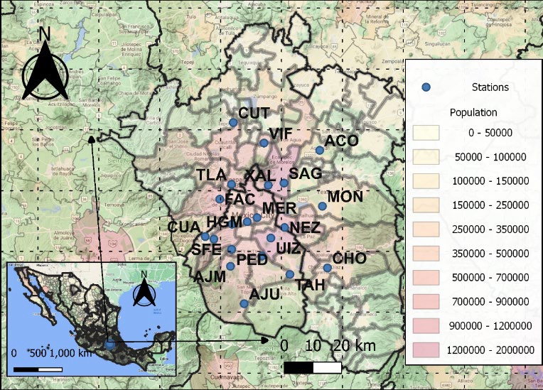
Fig. 1 Mexico City and location of air monitoring stations. The Palish yellow to red palette shows the total population by municipalities, while the green color displays the main green areas.
Statistical analysis and graphics were computed employing R language programming libraries [17]or all pollutants, and non-parametric statistics were employed for testing (p < 0.05); meanwhile, parametric statistics were used for meteorological data. The temporal and spatial trends were performed using the OpenAir package for R language [18]. For the meteorological variables, the period between 2017 and 2021 was analyzed to demonstrate its importance during the lockdown period. For pollutants data, the same periods between March 23 and May 20 were examined for each year of 2019 (pre-lockdown), 2020 (lockdown), and 2021 (post- lockdown). Table S2 in the supplementary material shows details of the official decisions regarding human activities control.
Influence of potential sources
A polar plot module from the OpenAir R package was employed to provide information about possible source characteristics only during the COVID-19 lockdown. Briefly, a Generalized Additive Model (GAM) was employed to show the pollutant concentration variation with wind speed and wind direction in polar coordinates. Then, through continuous surfaces calculated using the isotropic smoothing technique, one avoids the potential difficulty of handling two variables on different scales; details of this model applied to airplane emissions are described elsewhere [19]. The GAM can be explained by Equation 1:
where Ci is the ith concentration of pollutant in the time series, sj(xij) is a smooth function of covariate p with n as the total number of covariates, and εi is the ith residual. The smoothing parameter is based on a simple spline regression [20,21].
According to the wind speed and direction, the distance of the O3 emission sources was calculated, assuming that ozone concentration was not depleted from the source up to reaching the measurement site during the peak concentrations. We considered the duration of the ozone peak concentrations as 3 hours (13:00 to 16:00). This simple approach allowed us to determine the possible origin of ozone formation or emission in Mexico City and correlate the location with stationary or traffic-related emission of air pollutants
Correlation analysis
This work presents several correlation analyses between all data pairs through a correlation matrix plot. The correlation matrixes are coded by ellipses as a representation of scatter plots. The ellipses have a slope, positive or negative, accordingly. For zero correlation, the shape becomes a circle, and the color of the shapes reflects the value of the correlation parameter (r) in terms of percentage. The correlation analysis aimed to find the potential influence of criteria air pollutants in the dispersion of COVID-19 disease. A delay of five days in the number of infections by SARS-CoV-2 paired with the pollutant data was considered because five days is the average time in which symptoms appeared in an infected person [4]. Mobility data was obtained from the COVID-19 Community Mobility Reports from Google Inc. [22]. The number of infections and deaths due to COVID-19 was acquired from the National Council of Science and Technology of Mexico [23].
Results and disussion
Meteorology
The variation in meteorological variables influences the behavior of air pollutants, i. e., wet deposition, ozone formation enhancement due to high solar radiation, dry deposition, wind removal, etc.; however, human activities also impact the emission and distribution of pollutants. Our results showed no statistical differences (ANOVA and t-test, p > 0.05) in the meteorological variables from 2017 to 2021, and they had the same trends in all years analyzed. In this regard, during the COVID-19 lockdown period, any variations in air pollution concentration were mainly due to changes in anthropogenic activities. Fig S1 in the supplementary material displays this analysis visually.
Spatial and temporal variations of criteria air pollutants
The temporal and spatial variation of criteria air pollutants is visually resumed in Fig. 2. The figure shows the mean concentration of criteria air pollutants only between March 23 and May 20 for years 2017, 20181 2019 (pre-lockdown), 2020 (COVID-19 lockdown) and 2021 (post-lockdown). Most locations' temporal behavior was similar because they followed the same trends. However, we focused the analysis comparing pre- lockdown, lockdown, and post-lockdown; in this regard, most pollutants decreased their concentration from the pre-lockdown to the lockdown period, followed by increasing concentration during the post-lockdown.
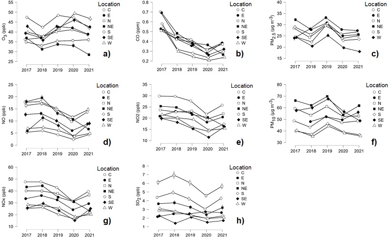
Fig. 2 Spatial and temporal variation of criteria air pollutants between March 23 and May 20 from 2017 to 2021.
The decrease in concentration between 2019 and 2020 was negatively correlated with mobility. According to the Mobility Secretary of Mexico City [24] mobility was reduced by 67% during the COVID-19 lockdown. In addition, industrial emissions did decrease and contributed to the improvement in air quality. Briefly, the reductions between pre-lockdown and lockdown were 29% (CO), 55% (NO), 25% (NO2), 28% (SO2), 25% (PM2.5), and 14% (PM10). In the case of ozone, its behavior was contrary, and its concentration increased by 19% (west of Mexico City) or remained unchanged (North, east, and south of Mexico City). Once the imposed COVID-19 lockdown finished, human activities returned gradually to the pre-COVID-19 situation. During 2021 almost all criteria air pollutants returned to similar levels to 2019. No significant differences (Kruskal-Wallis, p > 0.05) were found in pollutants concentration between the pre-lockdown and post- lockdown periods, except ozone and PM2.5, whose concentration was statistically higher (Mann-Whitney U, p < 0.05) in 2021 compared to 2019.
A basin describes the orography of Mexico City with multiple mountain systems over the east, west, and the highest mountain chains located south of the MAMV [16]. This topography and the prevailing wind conditions make the MAMV a region with high levels of air contamination due to stagnant conditions fostered by the heat island phenomenon [25]. Spatial trends of criteria air pollutants were similar for all regions of Mexico City. With a few exceptions, for most contaminants, the north, northeast, and center had higher pollution concentrations than the east, west, south, and southeast (Mann-Whitney U, p < 0.05). Again, ozone displayed a different behavior that will be discussed in a posterior section. The geographical characteristics of Mexico City explain the spatial trend since industry dominates the north and northeast of the city. At the same time, the center had the highest mobility at all times compared to the rest of Mexico City [26]. Meanwhile, the south and southeast are characterized by residential, commercial, and essential ecological reserves for Mexico City.
Ozone, temporal, and spatial variations
Ozone, contrary to other air criteria pollutants, depending on the location, concentration remained unchanged or increased (+19%, west) from pre-lockdown to COVID-19 lockdown periods. During the post- lockdown, the pollution levels decreased for most sites, even to concentrations below (-11% south) the observed before the pandemic. Table 1 shows the percentage of ozone concentration change between pre-lockdown, lockdown, and post-lockdown periods while Fig 2a shows the temporal and spatial trends.
Table 1 Percentage change of ozone concentration between March 23 and May 20 of 2019 (pre-lockdown), 2020 (COVID-19 lockdown), and 2021 (post-lockdown).
| Location | Change in [O3] (%)2020 – 2019 Lockdownvs pre-lockdown | Change in [O3] (%)2021 – 2020 Post-lockdown vs lockdown | Change in [O3] (%)2021 – 2019 Post- vs pre-lockdown |
| N | +1% | +1% | +2% |
| NE | -2% | -14% | -16% |
| W | +19% | -6% | +12% |
| C | +3% | -6% | -3% |
| E | -2% | -8% | -9% |
| S | -3% | -11% | -13% |
| SE | +9% | -8% | +1% |
As shown in Table 1, ozone concentration did not change significantly during the COVID-19 lockdown in Mexico City for most sites, as reductions were observed for the northeast, east, and south between 2% and 3% concerning the same period a year before the pandemic and a slight increase in the north and center of the city. These results were outstanding since the mentioned sites had strong vehicular and industrial VOC sources, which are potential ozone precursors. On the other hand, the west and southeast of the city had a significant increase in ozone pollution, which was also surprising since those sites mainly had domestic and biogenic VOC sources. In this regard, results suggested that biogenic and domestic VOC sources can be responsible for the ozone episode during the COVID-19 lockdown.
There are other possibilities to explain the observed trend for ozone during the COVID-19 outbreak. Some authors [11] showed a shift from a VOC-limited region to a NOx- limited area and stated that domestic VOC emissions contributed to ozone formation. However, other studies [27] have referred that domestic emissions significantly impact indoor pollution rather than exterior spaces. In this way, it is complicated that VOC from indoor spaces compensated for the diminution in anthropogenic VOC emissions due to low mobility and reduced human activities. The Mexican inventory of emissions sources [28] categorizes them as area (domestic, small commerce, agriculture, and non-regulated), natural (biogenic emissions from plants, animals, and microorganisms), mobile (vehicular), and punctual or fixed (industrial and big commerce) sources. According to this inventory, up to 2018, 69% of total emissions were related to area sources, followed by mobile (20.9%), punctual (7%), and natural (3.1%). If we consider that during the COVID-19 lockdown, most emission sources declined, except domestic, then natural and area sources were responsible for the ozone levels observed at the west and southeast of Mexico City.
Since there are no VOC measurements in Mexico City for the studied periods, corroborating the increase in VOC emissions that explain the increment in ozone concentration during COVID-19 lockdown results is complicated. Besides, there are reports that several urban sites displayed improvements in ozone pollution due to decreased NOx emissions produced from reduced human activities [29], which is consequent and does not support the behavior observed in Mexico City. In this regard, we suggested ozone formation from biogenic VOC (BVOC) even in a low-NOx and low anthropogenic VOC scenario. As data showed, NOx emissions and mobility decreased significantly during the COVID-19 lockdown; however, BVOC emissions did not change abruptly since vegetation response to external factors (i.e., stress due to anthropogenic emissions) was not so fast [30] and remained at the same levels compared to previous years. In the case of low anthropogenic VOC emissions and low NOx, BVOC could compensate for the reactants needed to form ozone during the lockdown. In other words, under pre-pandemic conditions, plants produced BVOC to combat anthropogenic VOC stress through radical reactions. However, during the lockdown, anthropogenic VOC decreased drastically and BVOC remained unchanged; as consequence, BVOC would participate in the formation of ozone rather than neutralizing anthropogenic emissions.
In this regard, measurements of anthropogenic VOC and BVOC markers are necessary to correlate them with ozone formation, which for now, is out of our scope. However, in the next section, we employed a visual approach to link the ozone formation during the COVID-19 lockdown with BVOC emissions, assuming that those were mainly emitted from green areas in Mexico City.
Ozone pollution sources
The bivariate polar plots for ozone were obtained for each location of Mexico City, considering only the lockdown period. In these plots, the ozone concentration was classified according to a wind vector which includes speed and direction. From the latter, it is possible to discern where ozone was transported and presumably formed if ozone is assumed not to be destroyed during the measurements. Fig. 3 displays the bivariate polar plots for ozone in Mexico City during the COVID-19 lockdown. The color scale goes from blue to red, representing low to high ozone concentrations. As can be seen, the lowest ozone pollution was local in all sites of Mexico City, as the lowest concentrations were in the center of each plot (Station's location). In contrast, the highest concentrations were transported from sources around the measurement site.

In Fig. 3 can be observed that in the north of Mexico City, ozone pollution was mainly transported from sources located to the southeast of Mexico City. Meanwhile, for the northeast of Mexico City, pollution came from the southwest, and there was a punctual source in the northeast. In the case of the city's west, ozone was transported from the east; the same for the center and east of Mexico City, although the center and the east had sources from the southwest too. The city's south had ozone transport mainly from a location at the northeast and distant sources from the south. Finally, the southeast of Mexico City presented ozone pollution coming from all directions except the northwest.
Our evidence that BVOC emissions were related to ozone formation during lockdown was based on the potential emission sources identified with the polar plots. The estimation considered that ozone was formed mainly where the ozone peak concentrations were located, then according to the wind speed direction and assuming that ozone was not depleted during measurements, the distance to the source was obtained. This approach identified that ozone peak concentrations during the COVID-19 lockdown were located over green areas close to usually transited roads. An example of this analysis is given in Fig. 4, where a representative monitoring station from the west of the city displayed that ozone peak concentration was transported from the Prado de la Montaña park and Carlos Lazo Avenue, both situated to the east. Also, a significant contribution was located northeast of the station where Alameda Poniente Park and Constituyentes avenue are situated. Finally, a dispersed source was located west, related to the park La Mexicana and the Mexico-Toluca Road.
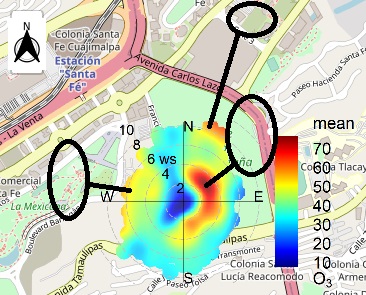
Fig. 4 Bivariate polar plot and source identification for ozone peaks concentrations in SFE air monitoring station located to the west of Mexico City.
The previous approach was consistent in almost all air monitoring stations except the north and northeast stations. However, some of the maximum ozone concentrations were correlated to main roads in those cases. For example, at the VIF station situated to the north of Mexico City, ozone was transported from Jaguares Park and Zarzaparrillas Road from the west of the station. Still, from the south of the station, ozone was transported from the intersection of Yutes street and Coacalco Boulevard. A similar scenario was obtained for the CUT station located north of the city, where ozone peak concentration came from the south of the station toward Insurgentes Avenue and Cuatitlan-Teoloyucan Road. In this way, despite these exceptions, ozone pollution was related to large green areas and heavy traffic roads for most of the monitoring stations. Similar and more refined analyses have been employed in other cities. For example, Li and Cheng [30] used satellite observations and deep learning not only to identify hot spots of ozone emissions but to model the spatial and temporal variation of the tropospheric ozone concentration in urban centers in China. Other authors developed a model that not only predicts ozone's spatial and temporal variation but can also estimate the concentration in locations without ozone measurements. These results are similar to the findings in other studies, as they observed an increase in ozone concentration attributed to biogenic emissions of VOCs, as discussed in the next paragraph.
In addition, the importance of BVOC emissions in ozone formation has been highlighted in recent studies. For example, some authors [31] have identified that ozone related to BVOC usually is increased by five ppb; however, its contribution could be even 30 ppb in some locations. Also, in Los Angeles in the United States, BVOC emissions from urban greening programs contributed to ozone and SOA formation with significant effects on urban air quality [32]. Finally, Shaobo Zhang and collaborators [33] modeled the impact of BVOC emissions on Ozone air quality in the Sichuan Basin in Southwestern China. They found that BVOC is critical in ozone episodes, mainly during summertime when solar radiation is the highest. In this last study, authors also found that BVOC emissions contributed substantially to ozone concentrations and elevated peak O3 levels up to 36.5 µg m-3 in the basin. This result is relevant because a similar situation could occur in Mexico City since it is in a basin surrounded by mountain systems which difficult the dispersion of air pollutants.
We do not intend to attribute solely to BVOC emissions the ozone episodes in recent times or even during the anomaly of the ozone concentration due to the COVID-19 lockdown. However, we should emphasize that natural emissions of BVOCs usually respond to external stress (i. e. anthropogenic air pollution) to protect themselves through organic radical neutralization during the day, aided by OH radical chain reactions. In other words, the high levels of anthropogenic emissions have caused over time BVOC emissions also rise. Without the first ones, the latter would not participate in ozone formation.
Correlation matrixes
Correlation analysis is a functional and commonly used analysis technique to evaluate how variables relate to one another; however, it can be difficult to understand relationships when many different variables are present. This work presents several correlation analyses between all data pairs through a correlation matrix plot. Fig. 5 shows the correlation matrixes for different time intervals a) considering only the COVID-19 lockdown period in the MAMV and b) considering all data since the first case of SARS-CoV-2 was reported in Mexico City. The correlations in Fig. 5 are coded by ellipses shapes as a visual representation of scatter plots. With a perfect correlation, the shape turns into a line with a positive or negative slope accordingly. Meanwhile, for zero correlation, the shape becomes a circle; the shape's color also reflects the value of the correlation parameter (r), and the r value is shown in percentage for each shape.
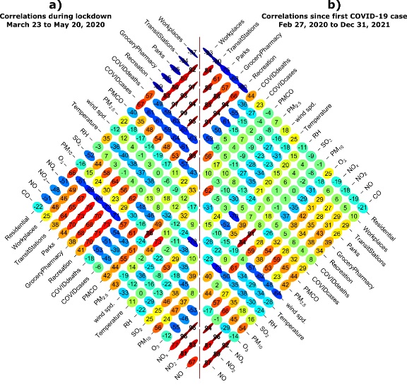
Fig. 5 Correlation matrixes of air criteria pollutants and the number of SARS-CoV-2 infections. Oval shapes turn into lines as correlation increases. The correlation parameter is shown in two-digit form. a) The lockdown correlation matrix only contemplates data from March 23 and May 20, 2020. b) contemplate the whole years since the first COVID-19 case was reported.
There were limitations when correlations on the COVID-19 lockdown period were done (Fig 5a) as the data collected in this period was relatively short; however, valuable information can be extracted from this correlation matrix. First, although vehicular mobility decreased during this period [12-14], pollutants associations remained unchanged from historical results (2015 - 2021 analyzed this work). We showed that for most pollutants (NO, NO2, NOx, CO, and PM2.5) sources were linked to vehicular emissions, as usual, negative and significant correlations (p < 0.001) were found between O3 and nitrogen oxides. Meanwhile, PM2.5 and PM10 were also strongly correlated. Concerning the number of COVID-19 infections only during the lockdown period, we found a strong positive correlation with O3 concentration and significant negative correlations with SO2, NO2, and NOx. We attribute those to restriction measures imposed by the Mexican government in terms of mobility. As discussed earlier, the decrease in nitrogen oxides and particle matter concentration was associated with low vehicular mobility. Then also, the number of infections was limited by the traffic reduction. Other studies [5-9] have found associations between NO2, CO, and PM2.5 during their respective confinement periods, concluding that air pollution may significantly influence disease dissemination. Our results did not reflect the same as the first cases in Mexico City were detected long after spreading the virus in Asiatic and European countries.
Once we considered an extended period (Fig 5b, since the first COVID-19 case was reported until the last day of 2021), we found that the number of infections had a positive and significant correlation (p < 0.001) with nitrogen oxides (r < 0.32) and CO (r = 0.32). On the other hand, significant (p<0.001) and negative correlations were found with ozone (r = -0.26) and temperature (r = -0.30). Particle matter remained not correlated with the number of infections. Although particle composition is highly complex and may include viruses among their constituents, the lack of correlation between PM and the number of infections was evidence that air pollution was not related to the spreading of the disease. Here we hypothesized that indoor conditions were more critical in spreading the virus, and exterior pollution did not reflect clearly how the number of infections was changing over time. However, we consider that the changes associated with mobility had a more significant impact on the disease spreading.
Conclusions
The COVID-19 pandemic brought an extraordinary opportunity to determine the behavior of criteria air pollutants under low anthropogenic influence. We found that most criteria air pollutants decreased their concentration substantially in correlation with reduced human mobility. For ozone, a different scenario took place, and its concentration remained invariant and even increased in some locations of Mexico City during the COVID-19 lockdown period. The spatial and temporal analysis showed that for all pollutants, independently of the time, the north, northeast, and center of Mexico City had the highest concentrations. For ozone, the west and southeast were the most polluted areas.
Meanwhile, the source identification by bivariate polar graphs allowed us to correlate the peak ozone concentrations during the lockdown with green areas and high vehicular transited roads. It was possible to identify that even under low NOx and assuming low anthropogenic activity, the emission of VOC significantly contributed to ozone contamination in urban areas. The potential VOC sources during the lockdown were possibly due to biogenic emissions or area sources, like domestic. It is important to remark that although BVOC emissions had an essential contribution to ozone formation during the COVID-19 lockdown, this result reflected how anthropogenic emissions had caused high stress over natural sources. We recommend that the authorities make informed decisions when implementing urban greening programs or reforestation plans since BVOC emissions can significantly impact the formation of tropospheric ozone. Also, it is recommended to consider the routine measurement of anthropogenic and biogenic VOC markers to understand better the chemistry in complex urban atmospheres like Mexico City.

