Definitions

Meteorological droughts (MD) are recurrent extreme climatic events that occur in any area of the country, including humid regions. They are characterized by scarce or lower than normal precipitation, occurring for several months or years. MDs are dry periods, as opposed to the permanent dryness of arid regions. Due to the constant increase in water demand for all uses and the negative effects of climate change, droughts have become more severe and their impacts are more noticeable and prolonged (^{Mishra & Singh, 2010}; ^{Fuchs, Svoboda, Wilhite, & Hayes, 2014}).

Given that in some water systems the period between the shortage of precipitation and its detection as a deficit varies considerably, droughts have been established as a phenomenon on multiple scales over time. Meteorological, agricultural, hydrological and socio-economic droughts are defined when deficits occur in rainfed agriculture, irrigation, generation of hydroelectric energy, municipal and industrial water supply, as well as when economic, social and environmental impacts are quantified (^{Pandey, Sharma, Mishra, Singh, & Agarwal, 2008}; ^{Vicente-Serrano, Beguería, & López-Moreno, 2010}; ^{Fuchs et al., 2014}).

In general, MDs are a regional phenomenon characterized by three dimensions: severity or intensity, duration and surface extension (^{Tsakiris & Vangelis, 2005}). This has led to the development of various drought indices for their detection and monitoring, which analyze separately or jointly the dimensions cited and allow the objective comparison between MDs that occur in dissimilar climates and help in the formulation of mitigation plans of their negative effects (^{Pandey et al., 2008}; ^{Vicente-Serrano et al., 2010}; ^{Fuchs et al., 2014}).

Common MD Indices

The first meteorological drought index that has been broadly used both in the U.S.A. as well as in other countries was the PDSI (Palmer Drought Severity Index), presented in the mid 1960s (^{Palmer, 1965}), so it is over 50 years old. It is a multivariate index that applies a soil moisture balance ( ^{Hao & Singh, 2015}) and uses monthly potential evapotranspiration and precipitation. But it is based on several fully empirical rules, as demonstrated by ^{Alley (1984}), and is quite sensitive to the period used for its coefficient calibration, as shown by ^{Karl (1986)}. It also does not allow the use of multiple time scales or drought durations. ^{Wells, Goddard and Hayes (2004)} developed a procedure for automatic calculation of the PDSI, which improves the regional comparison capacity of the index. ^{Pereira, Rosa and Paulo (2007)} used another water balance model to adapt the PDSI to the Mediterranean climate.

The next meteorological drought index with nearly universal application is the SPI (Standardized Precipitation Index), proposed in the early 1990s (^{McKee, Doesken, & Kleist, 1993}). This is multi-scalar in time and uses a probabilistic approach to analyze monthly precipitation, which has proven to be quite efficient. Such approach consists of two processes. The first analyzes monthly precipitation sequences as moving sums, according to the study duration of the droughts, which ranges from 1 to 72 months. In the second process, the formed sequences are fitted with a probability distribution function (FDP) to estimate their probability of non-exceedance, which by means of a numerical approximation is transformed into a standard normal variable (Z). The negative values correspond to meteorological drought sequences and their types are defined as light, moderate, severe and extreme, with the value of Z = SPI ranging from 0 to -1.00, from -1.00 to -1.50, from -1.50 to -2.00 and when it is less than -2.00, respectively.

Recently, the SPEI (Standardized Precipitation Evapotranspiration Index) has been proposed by ^{Vicente-Serrano et al. (2010)} and ^{Beguería, Vicente-Serrano, Reig and Latorre (2014)}, which has a calculation similar to that of SPI, but uses a measure of the monthly climate balance based on the difference (d) between monthly precipitation and potential evapotranspiration, instead of just precipitation. Because the differences, d, are generally negative, some moving sums or sequences are less than zero, in which case the FDP used has three fitting parameters, and that of location (u) must be less than the minimum sequence. The creators of the SPEI found that the log-logistics FDP results in a good probabilistic modeling of the sequences. ^{Stagge, Tallaksen, Gudmundsson, Van Loon and Stahl (2015)} have suggested the FDP General Extreme Values.

An important advantage of the SPEI over the SPI lies in incorporating the potential evapotranspiration variable and the ability to consider possible effects of climate change on the severity of meteorological droughts, through modifying or altering the historical precipitation and average monthly temperature records by reducing the former and/or increasing the latter, as shown by ^{Vicente-Serrano et al. (2010)}.

^{Ma et al. (2014)} described deficiencies and limitations in the difference, d, used by the SPEI as an equation of the monthly climate balance and proposed the use of the calculated moisture deviation, d^, as named by ^{Palmer (1965)}. The latter is equivalent to the difference between the observed precipitation and precipitation estimated for normal climate conditions in the region (P^), which is calculated based on the results of a soil water balance. ^{Ma et al. (2014)} found that d and d^ respond differently to variations in precipitation and temperature, according to climatic conditions. For dry climates, they found that d-series are excessively dependent on temperature, leading to large and even abnormal deficits as potential evapotranspiration grows, which is unattainable as real evapotranspiration in times of low precipitation.

Fortunately, the difference, d^, shows low variability in relation to temperature while also retaining the influence of precipitation, and therefore it has better spatial behavior. ^{Ma et al. (2014)} processed the differences, d^, with the SPI probabilistic approach, to develop the Standardized Palmer Drought Index (SPDI). This index includes the theoretical salvageable part of the Palmer index, the computational efficiency of the SPI and reproduces the sensitivity of the SPEI to study probable climate changes.

Objective

This study has three objectives: (1) the operating procedure of the SPDI is presented in detail, which was recently proposed by ^{Ma et al. (2014)}; (2) SPDI results are compared to the preceding indices (SPI and SPEI) for three MD durations of 6, 12 and 24 months, which attempt to characterize the agricultural and hydrological droughts; (3) these comparisons are carried out in three climatological stations (Villa de Arriaga, Río Verde and Xilitla) in the state of San Luis Potosí, Mexico, which have extensive records (≥ 50 years) and are located in each of their three geographical regions: Potosino Plateau, Middle region, and Huasteca Region. Based on the results of the analysis, conclusions are formulated.

Soil water balance

The original Palmer index (PDSI) starts with a soil water balance (SWB), performed on a monthly basis using historical precipitation (P) and average temperature (Tt) records. The storage (S) of moisture in the soil occurs in two layers. The first surface can save (Ss _max) up to 25 millimeters in water depth and the second, which is deeper, has a capacity (Su _max) that depends on the physical characteristics of the soil and the depth of the roots of vegetation, ranging from 127 to 229 millimeters (^{Palmer, 1965}). Figure 1 shows the flow chart of the SWB.

Figure 1 Flow chart of the water soil balance of the Palmer index (PDSI). 

Moisture cannot be extracted (or stored) in the deep layer (Su) until all the available moisture in the surface layer (Ss) is taken (or recharged). Potential evapotranspiration (PE) is estimated with the Thornthwaite method, which is presented next. The losses from soil (L) due to PE occur when PE> P, where P is precipitation. Evapotranspiration losses from the surface layer (Ls) occur at a potential level, while those from the deep layer (Lu) depend on the initial moisture content, PE and the storage moisture in both soil layers, designated by AWC (available water capacity = Ss _max + Su _max). Then, when PE > P, we have (^{Palmer, 1965}; ^{Alley, 1984}):

In the previous equations, Ss and Su are the moisture contents stored in each soil layer at the beginning of the respective month. The SWB of the Palmer method considers runoff (RO) to only occurs when the two layers of soil reach their total storage capacity (AWC) and is equivalent to the surplus of P minus the PE (availability) in the month, after filling both soil layers (ΔSs and ΔSu).

The concept of PE only occurs, according to its definition, when vegetation is actively growing, so that in arid climates it will not occur during the dry season, and in cold climates it will not occur during the winter. Then, the current or real evapotranspiration (ET) occurs when PE > P and is equal to:

Climatically normal monthly precipitation

As part of the SWB of the Palmer method, three additional terms are calculated with a potential or maximum level: recharge (PR), losses (PL) and runoff (PRO). The potential recharge for the month is defined as the amount of water necessary to bring the soil to its field capacity, therefore, this is equal to (^{Palmer, 1965}; ^{Alley, 1984}):

where Ss and Su are the values from the previous month. Potential losses are considered equal to the amount of moisture that can be lost from the soil due to PE when there is no precipitation; therefore they are:

Finally, regarding the potential runoff (PRO), potential precipitation (PP) is assigned to this value, which ^{Palmer (1965)} assigns to the value of AWC, less than potential recharge (PR). For the above:

In the previous equation, originally used by ^{Palmer (1965)}, it is obvious that the potential precipitation (PP) has a physically weak or scarce relation with the assigned value of AWC and therefore Palmer later suggested using the PP, equal to three times the average monthly precipitation (P-j). This modification was taken into account by ^{Pereira et al. (2007)}.

The four calculated potential values (PE, PR, PL and PRO) are used to calculate four coefficients (alpha, beta, gamma and delta) that are quotients of average values, which depend on the climate of the area that is being studied. They are:

where j ranges from 1 to 12, representing the month counter, and the average quantities are calculated with i annual values, which go from 1 to NY number of years on record (> 30). The above SWB coefficients are used to calculate CAFEC precipitation (climatically appropriate for existing conditions, named by ^{Palmer (1965)} designated by P^, that is:

The precipitation, P^, that is climatically appropriate for the existing conditions is an estimate from the SWB, which is equivalent, according to ^{Ma et al. (2014)}, to the minimum amount of precipitation necessary to maintain soil moisture under normal conditions in a certain region. According to Equation 14, it corresponds to the sum of real evapotranspiration, groundwater recharge and direct runoff, minus the change in moisture storage in the soil (^{Palmer, 1965}; ^{Alley, 1984}).

Moisture Deviation

The differences, d^, between monthly precipitation P and P^ in each month recorded are called moisture deviation (moisture departure) and corresponds to (^{Palmer, 1965}):

As indicated, ^{Ma et al. (2014)} processed the differences, d^, with the probabilistic SPI approach to develop the SPDI.

Monthly Potential Evapotranspiration

The Thornthwaite criterion estimates the PEji, in millimeters, of month j of year i, with the following empirical equation (^{Mather, 1977}; ^{Campos-Aranda, 2005}; ^{Xu, Singh, Chen, & Chen 2008}):

where Fc is a corrective factor function of the latitude of the site and ndm is the number of days of the month. Its formula is:

where N is the maximum sunlight or maximum number of hours with average monthly sunshine. For its estimation in the Mexican Republic, ^{Campos-Aranda (2005)} proposed the following empirical expression:

where nm is the number of the month, with 1 for January and 12 for December; A and B are constants functions of the latitude (LAT) of the site, in degrees, with the following expressions:

In Equation (16), Ttji is the monthly average temperature in °C, IC _i is an annual heat index, equal to the sum of the 12 monthly indices, which are:

Finally, in Equation 16 the exponent m is a function of IC _i with the following empirical expression:

For values of Ttji greater than 26.5 °C the IC _i has no influence, so the PEji is only a function of Ttji and is tabulated (^{Campos-Aranda, 2005}). The tabulation values cited can be represented by a line when Ttji varies from 26.5 to 28.0 °C and by a second-degree polynomial when Ttji is greater. These equations are:

Fitting of the Log-Logistic Distribution

Having calculated the differences, d^, with Equation 14, a chronological series is obtained of 12 by NY elements, being NY the number of years in the record processed. Then, these series are used to form sequences, such as moving sums of size k in months, equal to the duration of the drought that is being studied, commonly the following: 1, 3, 6, 9, 12, 18, 24, 30 and 36 months. For example, for k = 3 the first sequence will be the sum of the first, second and third value of d^, the second sequence will be the sum of the second, third and fourth value of d^ and so on until the last sequence (ns) that will be formed with the sum of the antepenultimate, penultimate and last value of d^. Therefore, the number of sequences (ns) that can be formed will be equal to:

The formed sequences will be designated by Dlk with l varying from one to ns. For the fitting of an FDP to the formed sequences, ^{Ma et al. (2014)} tested four probabilistic models: log-normal, Pearson type III, log-logistic and generalized extreme value distribution (GVE), recommending the latter, fitted with the L-moments method. For the case of the climatic information processed in this study, the use of the GVE distribution did not lead to a fitting that fulfills the condition that the location parameter (u) be lower than the magnitude of the minimum sequence (Dmink), therefore, the FDP log-logistics (LL3) was used, suggested by ^{Vicente-Serrano et al. (2010)} and verified by ^{Beguería et al. (2014)} for its use with the SPEI. The LL3 function is equivalent to the generalized logistic distribution through an adequate relation of parameters (^{Rao & Hamed, 2000}). The equation for the accumulated probability distribution function F(x) of the LL3 distribution is (^{Haktanir, 1991}):

where γ > 0, α > 0 and u < x _mo are the parameters of form, scale and location, whose values can be estimated with various statistical procedures. x _mo is the minimum observed datum (Dmink). ^{Ahmad, Sinclair and Werritty (1988}) found that the probability-weighted moments (PWM) method (βs), developed by ^{Greenwood, Landwehr, Matalas and Wallis (1979)}, is the most robust, as well as being a relatively simple and direct procedure. According to ^{Stedinger, Vogel and Foufoula-Georgiou (1993)}, the biased estimators of β_s must be used when fitting an FDP at a single site, and quantiles are estimated with it, because then their predictions have a lower mean squared error. These moments are calculated with the following two expressions (^{Hosking, 1990}; ^{Haktanir, 1991}; ^{Stedinger et al., 1993}; ^{Vicente-Serrano et al., 2010}:

where:

where l is the counter of sequences whose number is ns. Dlk are the sequences in an ascending order D1k≤D2k≤⋯≤Dnsk. ^{Beguería et al. (2014)} have suggested using the unbiased βs when the biased estimators do not lead to a numerical solution. The equations for estimating the three fitting parameters of the LL3 distribution are (^{Haktanir, 1991}):

where Γ(·) is the factorial function Gamma, which was estimated with the Stirling formula (^{Davis, 1972}), this is:

Having calculated the three fitting parameters (u, σ, λ), Equation 26 is applied with x=Dlk to estimate the probabilities of non-exceedance F(x) that correspond to each moving sum of duration k.

Calculation of the SPDI Values

Finally, in accordance with ^{McKee et al. (1993)}, the rational numerical approximation developed by ^{Zelen and Severo (1972)} is used to convert F(x) into the normalized standard variable Z of zero mean and unit variance, which defines the SPDI that is sought; their equations are:

where:

Processed Climatic Records

The state of San Luis Potosí is divided by their common watershed dividing Hydrological Regions No. 37 (El Salado) and No. 26 (Pánuco), as shown in Figure 2. The former region has an arid climate in the area known as Altiplano Potosino. In contrast, the Potosino portion of the Pánuco River basin is hot-humid; it is known as the Huasteca Region and begins approximately at the meridian 99° 30' W.G. This transition of climates creates a third geographic zone in the state, called Middle Zone, which has a temperate climate.

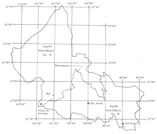
Figure 2 Geographic location of the three climatological stations processed in the state of San Luis Potosí, Mexico. 

In each of these three geographical zones, climatological stations were identified with largest number of records and the least number of missing monthly data of precipitation and average temperature. The following three stations were selected: Villa de Arriaga, Río Verde and Xilitla. In each of them, the few missing rainfall data were considered equal to the monthly mode, estimated based on the fitting of the Mixed Gamma distribution to all available monthly values (^{Campos-Aranda, 2005}). The few missing average temperature data were estimated with an interpolation procedure that took into account the trend observed in the month before and after the missing value.

The average monthly precipitation (mm) and average temperature (°C) values of each climatological station studied are listed in Table 1, as well as the respective recording periods. At the Villa de Arriaga station in the period from 2010 to 2014, average monthly temperature values were used, because its available records covered until 2009, when they were processed by ^{Campos-Aranda (2017)}. Table 1 shows the monthly average calculated potential evapotranspiration (PE _j ), based on the Thornthwaite method (Equations (16) to (24)). Figure 2 shows the location of the three climatological stations studied in the state of San Luis Potosí, Mexico.

Homogeneity Tests Applied

Based on the complete precipitation and average monthly temperature records, annual values were calculated. Based on these series, a statistical quality analysis was performed, for which the following seven tests were applied, one general and six specific: (1) Von Neumann, which detects decreased randomness by unspecified deterministic components, (2) Anderson and (3) Sneyers, which identify persistence, (4) Kendall and (5) Spearman, which detect trend, (6) Bartlett, which tests variability and (7) Cramer to identify changes in the mean. In all tests, a level of significance (α) of 5% was used. The statistical tests cited can be found in ^{WMO (1971)}, ^{Buishand (1982)} and ^{Machiwal and Jha (2008)}. The results of these tests are shown in Table 2, in which NH and H mean non-homogeneous and homogeneous series or record, respectively.

Regarding the annual precipitation (P), the records from Villa de Arriaga and Río Verde show persistence, detected even with the von Neumann test. Since persistence is a statistical component of the time series, analyses aimed at quantifying meteorological droughts can continue, given that the three records show no trend or changes in the mean, that is, loss of homogeneity.

The opposite occurred with annual average temperature (Tt) records, which are totally non-homogeneous since they present persistence, an upward trend and a change in the mean. Accepting that this loss of homogeneity is associated with climate change, these records can be processed, and the effects of the upward trend will be reflected in the monthly estimates of potential evapotranspiration, with Equations 16 to 24.

Relevant aspects of the computer program

The program designated by SPDI3 consists of three modules that were generated successively and thus were incorporated. In subprogram SPDI1, the SWB was developed based on Equations 1 to 15, which was completed when it succeeded in reproducing the values in Table 1 on page 10 of ^{Palmer's paper (1965)}, which presents three years (1933 to 1935) of a SWB performed in Central Iowa using Ss _max and Su _max equal to 1.0 and 9.0 inches, and starting with AWC equal to 10.0 inches. This module, called SWB, concludes with the calculation of moisture deviation (d^) with Equation 15, in metric decimal system; estimating the potential evapotranspiration (PE) by means of Equations 16 to 24. The code of the first module, which turned out to be the most complex to program, is available in BASIC language, from the author.

An interesting aspect of this first module is establishing the initial soil moisture conditions in the first year of records. This was resolved by trial and error, assigning values to Ss and Su in January and contrasting them with those of December of that year; when they were equal, the problem was solved. For subsequent years, the December values of a year are used as the initial values for January of the following year. Magnitudes of 25 mm for Ss _max and 150 mm for Su _max were adopted. Table 3 shows the pairs of values calculated by trial and error for Ss _inic and Su _inic, in the first year of records, as well as the sets of coefficients of the SWB obtained for each of the three climatological stations processed.

The subprogram SPDI2 incorporates the second module, in which the moving sums of duration k, in months, are calculated to form the sequences Dlk, whose basic statistical parameters (mean, standard deviation and coefficient of asymmetry) and minimum and maximum values are quantified. This module includes the fitting of the LL3 distribution to the formed sequence Dlk by means of Equations 25 to 32, and ends with the application of Equation 26 to estimate the probabilities of non-exceedance PX ≤x of each element in the sequence. Relevant results of this module are the shape, scale and location parameters of the LL3 function.

Next, the SPDI3 program is completed with the third module, which calculates the SPDI values by only transforming its probabilities of non-exceedance to standard normal variables (Z), by means of Equations 33 to 36. In addition, two statistical parameters of SPDI = Z are calculated, the mean and its variance, as well as its number of negative elements. These quantities are actually measurements of goodness of fit, since their values must be zero, one, and half the number of sequences formed (ns). The extreme minimum value of the SPDI is also detected. Finally, in this module the number of light, moderate, severe and extreme droughts is counted, corresponding to the number of SPDI values between 0 and -1.00, from -1.00 to -1.50, from -1.50 to -2.00 and that are less than -2.00, respectively.

Contrasts of the SPDI

Based on the SPDI3 program, the historical precipitation and average monthly temperature records from the three climatological stations in dissimilar climatic locations are processed for the three drought durations (k) established. The last three columns in Table 4, Table 5 and Table 6 show the results of the aforementioned program. Columns two, three and four present the results of the SPI index, which come from the calculations made by ^{Campos-Aranda (2017)}, and columns five, six and seven show the results of the SPEI index, applied using the Thornthwaite method (Equations 16 to 24).

Tables 4, 5 and 6 present four types of numerical values: [1] those associated with the sequences ( D l k ) or moving sums, (2) those related to the fitting of the mixed gamma (GM2) and log-logistic (LL3) distributions, [3] those corresponding to the statistical parameters of the SPI, SPEI and SPDI, which are indicators of the statistical quality of the fitting obtained and, therefore, reflect the accuracy of the results and [4] those associated with the four types of droughts studied.

Generalities

As seen in Tables 4, 5 and 6, the statistical parameters of the sequences formed with moving sums are quite different in each index. This is due to the fact that in the SPI they come from the monthly precipitation, in the SPEI from the differences (d) between the precipitation minus the monthly potential evapotranspiration, and in the SPDI from Palmer moisture deviations (d^).

Regarding the quality indicators of the fittings obtained, the SPDI was found to result in the best fittings in the three processed climatological stations, since their mean and variance are closer to zero and one. The worst fittings were those resulting from the SPI index. In general, the SPEI and SPDI indices tended to overestimate the number of droughts in the three climatological stations processed, and the SPI’s estimates were better for the 6- and 12-month durations.

Finally, regarding the percentages of each type of drought established by the three indices, all report similar values in order of magnitude, but they differ in a specific way for each duration of drought, mainly in relation to severe and extreme droughts.

Based on the results of Tables 4, 5 and 6, it can be deduced that the percentages of the less dispersed and more similar types of drought were obtained with the 12-month duration. Then, taking as a reference the percentages defined by the SPDI, they were compared with those of the SPI and the SPEI, and representative values were selected, adjusting these percentages to a sum of 50%. The Villa de Arriaga resulted in 33%, 11 %, 5% and 1% for light, moderate, severe and extreme droughts, respectively. The Río Verde station resulted in 34%, 11%, 4% and 1% and Xilitla resulted in 31%, 12.5%, 6% and 0.5%, respectively.

Definition of Periods of Drought

Figure 3, Figure 4 and Figure 5 present the graphs of the evolution of the SPDI index for each of the three climatological stations processed, for the duration of 12 months, which was found to be the most convenient for establishing representative values.

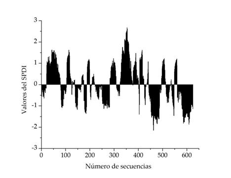
Figure 3 Evolution of the SPDI for 12-month durations in the Villa de Arriaga climatological station in the state of San Luis Potosí, Mexico. 

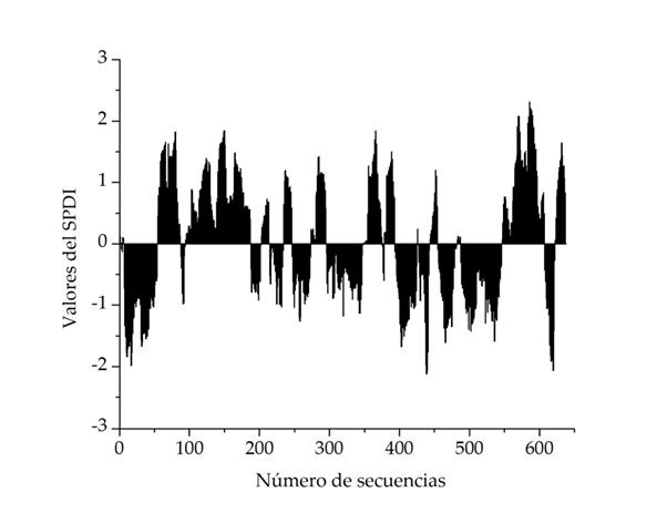
Figure 4 Evolution of the SPDI for 12-month durations in the Río Verde climatological station in the state of San Luis Potosí, Mexico. 

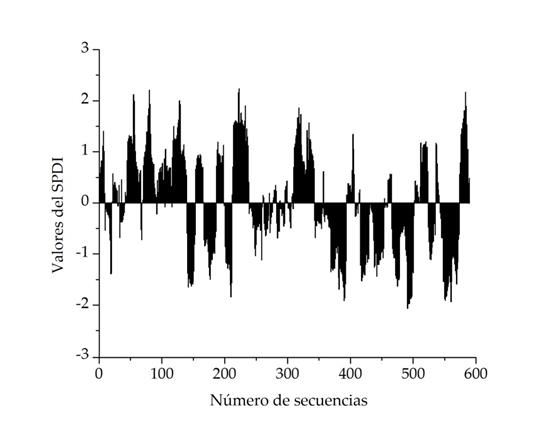
Figure 5 Evolution of the SPDI for 12-month durations in the Xilitla climatological station in the state of San Luis Potosí, Mexico. 

Figure 3 shows the most severe droughts in duration and magnitude occurred in the last drought period, which contains the extreme minimum value. The second event begins in sequence 443 (October 1999) and ends in 495 (February 2004), with the maximum event occurring in sequence 463 (June 2001). The dates in parentheses are obtained based on Equation 25, clearing NY, whose whole part defines the year by adding it to the beginning of the record, and its fractional portion is defined by multiplying it by 12, resulting in the respective month number. The most critical drought period, the last one, began in sequence 561 (August 2009) and ended in 625 (December 2014).

Figure 4 shows that the first drought was one of the most severe, which began in sequence 7 (June 1962) and ended in 54 (May 1966). The maximum event occurred in sequence 439 (June 1998).

From Figure 5, it can be deduced that the period with the most severe drought was the antepenultimate one, which begins in sequence 466 (September 2004) and ends in 501 (August 2007). The extreme maximum event occurred in sequence 491 (October 2006).

REFERENCES

Ahmad, M. I., Sinclair, C. D., & Werritty, A. (1988). Log-logistic flood frequency analysis. Journal of Hydrology, 98(3), 205-224. [ Links ]
Alley, W. M. (1984). The Palmer drought severity index: Limitations and assumptions. Journal of Climate and Applied Meteorology, 23(7), 77-86. [ Links ]
Beguería, S., Vicente-Serrano, S. M., Reig, F., & Latorre, B. (2014). Standardized Precipitation Evapotranspiration Index (SPEI) revisited: Parameter fitting, evapotranspiration models, tools, datasets and drought monitoring. International Journal of Climatology, 34(10), 3001-3023. [ Links ]
Buishand, T. A. (1982). Some methods for testing the homogeneity of rainfall records. Journal of Hydrology, 58(1-2), 11-27. [ Links ]
Campos-Aranda, D. F. (2005). Estimación de la evapotranspiración y análisis de la precipitación. En: Agroclimatología Cuantitativa de Cultivos (pp. 65-120). México, DF, México: Editorial Trillas. [ Links ]
Campos-Aranda, D. F. (2017). Cuantificación de sequías meteorológicas mensuales: cotejo de cuatro índices en tres localidades de San Luis Potosí, México. Tecnología y Ciencias del Agua, 8(3), 159-172. [ Links ]
Davis, P. J. (1972). Gamma Function and related functions. In: Abramowitz, M., & Stegun, I. A. (eds.). Handbook of Mathematical Functions (pp. 253-296). New York, USA: Dover Publications. [ Links ]
Fuchs, B. A., Svoboda, M. D., Wilhite, D. A., & Hayes, H. J. (2014). Drought indices for drought risk assessment in a changing climate. In: Eslamian, S. (ed.). Handbook of Engineering Hydrology. Modeling, Climate Change and Variability (pp. 217-231). Boca Raton, Florida, USA: CRC Press. [ Links ]
Greenwood, J. A., Landwehr, J. M., Matalas, N. C., & Wallis, J. R. (1979). Probability weighted moments: Definition and relation to parameters of several distributions expressible in inverse form. Water Resources Research, 15(5), 1049-1054. [ Links ]
Haktanir, T. (1991). Statistical modeling of annual maximum flows in Turkish rivers. Hydrological Sciences Journal, 34(4), 367-389. [ Links ]
Hao, Z., & Singh, V. P. (2015). Drought characterization from a multivariate perspective: A review. Journal of Hydrology, 527, 668-678. [ Links ]
Hosking, J. R. M. (1990). L-moments: Analysis and estimation of distributions using linear combinations of order statistics. Journal of the Royal Statistical Society B, 52(1), 105-124. [ Links ]
Karl, T. R. (1986). The sensitivity of the Palmer drought severity index and Palmer’s Z-index to their calibration coefficients including potential evapotranspiration. Journal of Climate and Applied Meteorology, 25(1), 77-86. [ Links ]
Ma, M., Ren, L., Yuan, F., Jiang, S., Liu, Y., Kong, H., & Gong, L. (2014). A new standardized Palmer drought index for hydro-meteorological use. Hydrological Processes, 28(23), 5645-5661. [ Links ]
Machiwal, D., & Jha, M. K. (2008). Comparative evaluation of statistical tests for time series analysis: Applications to hydrological time series. Hydrological Sciences Journal, 53(2), 353-366. [ Links ]
Mather, J. R. (1977). The Climatic Water Budget. Exercise V. In: Thornthwaite, C. W., & Mather, J. R. (eds.) Workbook in Applied Climatology (pp. 29-44). New Jersey, USA: Laboratory of Climatology. [ Links ]
McKee, T. B., Doesken, N. J., & Kleist, J. (1993). The relationship of drought frequency and duration to times scales. Eight Conference on Applied Climatology Anaheim, California, USA. [ Links ]
Mishra, A. K., & Singh, V. P. (2010). A review of drought concepts. Journal of Hydrology, 91(1-2), 202-216. [ Links ]
Palmer, W. C. (1965). Meteorological Drought (Research Paper No. 45). Washington, DC, USA: U.S. Office of Climatology, US, Weather Bureau, Department of Commerce. [ Links ]
Pandey, R. P., Sharma, K. D., Mishra, S. K., Singh, R., & Agarwal, A. (2008). Drought characterization. In: Singh, V. P. (ed.). Hydrology and Hydraulics (pp. 761-792). Highlands Ranch, Colorado, USA: Water Resources Publications. [ Links ]
Pereira, L. S., Rosa, R. D., & Paulo, A. A. (2007). Testing a modification of the Palmer drought severity index for Mediterranean environments. In: Rossi, G., Vega, T., & Bonaccorso, B. (eds.). Methods and Tools for Drought Analysis and Management (pp. 149-167). Dordrecht, The Netherlands: Springer. [ Links ]
Rao, A. R., & Hamed, K. H. (2000). Generalized Logistic Distribution. Theme 9.2 (pp. 302-321). In: Flood Frequency Analysis. Boca Raton, Florida, USA: CRC Press . 350 p. [ Links ]
Stagge, J. H., Tallaksen, L. M., Gudmundsson, L., Van Loon, A. F., & Stahl, K. (2015). Candidate distributions for climatological drought indices (SPI and SPEI). International Journal of Climatology, 35(18), 4027-4040. [ Links ]
Stedinger, J. R., Vogel, R. M., & Foufoula-Georgiou, E. (1993). Frequency Analysis of Extreme Events. In: Maidment, D. R. (ed.). Handbook of Hydrology (pp. 18.1-18.66). New York, USA: McGraw-Hill. [ Links ]
Tsakiris G., & Vangelis H. (2005). Establishing a drought index incorporating evapotranspiration. European Water, 9(10), 3-11. [ Links ]
Vicente-Serrano, S. M., Beguería, S., & López-Moreno, J. I. (2010). A multiscalar Drought Index sensitive to Global Warming: The Standardized Precipitation Evapotranspiration Index. Journal of Climate, 23(7), 1696-1718. [ Links ]
Wells, N., Goddard, S., & Hayes, M. J. (2004). A self-calibrating Palmer drought severity index. Journal of Climate, 17(12), 2335-2351. [ Links ]
WMO, World Meteorological Organization. (1971). Standard tests of significance to be recommended in routine analysis of climatic fluctuations. Annexed III. In: Climatic Change. Technical Note No. 79 (pp. 58-71). Geneva, Switzerland: Secretariat of the World Meteorological Organization. [ Links ]
Xu, C., Singh, V. P., Chen, Y. D., & Chen, D. (2008). Evaporation and Evapotranspiration. In: Singh, V. P. (ed.). Hydrology and Hydraulics (pp. 229-276). Colorado, USA: Water Resources Publications. [ Links ]
Zelen, M., & Severo, N. C. (1972). Probability functions. In: Abramowitz, M., & Stegun, I. A. (eds.). Handbook of Mathematical (pp. 925-995). New York, USA: Dover Publications . [ Links ]
Received: December 12, 2017; Accepted: February 22, 2018
Este es un artículo publicado en acceso abierto bajo una licencia
Creative Commons