


Servicios Personalizados
Revista
Articulo
 texto en
  Artículo en XML
 Referencias del artículo
 Enviar artículo por email
Indicadores
-
 Citado por SciELO
 -
 Accesos
Links relacionados
-
 Similares en
SciELO
Similares en
SciELO
Compartir

 Permalink
Tecnología y ciencias del agua
versión On-line ISSN 2007-2422
Tecnol. cienc. agua vol.11 no.1 Jiutepec ene./feb. 2020 Epub 30-Mayo-2020
https://doi.org/10.24850/j-tyca-2020-01-01
Articles
Uncertainty in the evaluation of climate change impacts over two Mexican Catchments

1Consejo Nacional de Ciencia y Tecnología, El Colegio de San Luis, San Luis Potosí, México, javelazquezza@conacyt.mx
2Département du Génie de la Construction, École de Technologie Supérieure, Université du Québec, Montréal, Canada, magali.troin@etsmtl.ca
3HydroClimat, Toulon, France, magali.troin@hydroclimat.com
This study explores the uncertainties associated with general circulation model (GCM), emission scenarios and natural climate variability into estimates of climate change impacts over two Mexican catchments. The two selected catchments have contrasted climate patterns and hydrological regimes. Climate ensemble simulations from three GCMs under three SRES scenarios (B1, A1B, and A2) are considered to feed the physically-based semi-distributed SWAT hydrological model. The simulations cover the 30-year reference period (1971-2000) and two 20-year periods (2046-2065 and 2081-2100) in the future. For the set of hydrological indicators, the results show that the high flows are more prone to be influenced by the GCM uncertainty. A weak sensitivity of the hydrological indicators is observed to emission scenarios over the study catchments. We find that the uncertainty related to the natural climate variability should not be neglected in climate change impact studies, and appears, to some extent, to be as critical as the GCM and scenario uncertainties for high flows.
Keywords: Climate change impact; model chain; streamflow; uncertainty; natural variability; SWAT; Mexico
Este estudio investiga la incertidumbre asociada con el modelo de circulación general (MCG) al escenario de emisión y a la variabilidad natural del clima en la estimación del impacto del cambio climático en dos cuencas mexicanas. Las cuencas seleccionadas tienen diferentes climas y regímenes hidrológicos. Las simulaciones climáticas de tres MCG bajo tres escenarios de emisión (B1, A1B y A2) se usan para alimentar el modelo hidrológico SWAT, de tipo físico y semidistribuido. Las simulaciones cubren 30 años en un periodo de referencia (1971-2000) y dos periodos de 20 años en el futuro (2046-2065 y 2081-2100). Los resultados muestran que los caudales altos son más propensos a ser influenciados por la incertidumbre asociada con el MCG; además, los indicadores hidrológicos tienen una sensibilidad menor al escenario de emisión para las cuencas de estudio. Por último, la incertidumbre vinculada con la variabilidad natural no debe pasarse por alto en los estudios de cambio climático, ya que hasta cierto punto y para caudales altos puede ser tan crítica como la incertidumbre ligada con MCG y el escenario de emisión.
Palabras clave impacto del cambio climático; cadena de modelación; escurrimiento; incertidumbre; variabilidad natural; SWAT; México
Introduction
Climate change projections for Mexico and Central America suggest changes in precipitation and an increase in temperature that will affect the future availability of water resources in the region (IPCC, 2014). Table 1 shows some studies of climate change impacts on water resources in Mexican basins. The use of several General Climate Models (GCMs) allows the uncertainty related to the climate model in the evaluation of climate change impacts on water resources to be assessed. Recently Velázquez-Zapata, Troin and Dávila-Ortiz (2017), and Molina-Navarro et al. (2016) evaluated climate change impacts with five and six climate models, respectively. On the other hand, the work of Rivas, Güitrón and Montero (2011) combined outputs from 23 GCMs to obtain an averaged climate model simulation. However, Arnell and Gosling (2013) claimed that averaging model outputs lead to a loss of signal in precipitation (when estimated changes are of different sign) and to an underestimation of the spatial variability of the signal. Furthermore, none of the previous studies have considered the uncertainty associated with the natural climate variability (NCV). The NCV is estimated by repeating a climate change experiment using a given GCM several times, when only the initial conditions are changed by small perturbations (Braun, Caya, Frigon, & Slivitzky, 2012). In that aspect, Deser, Knutti, Solomon and Phillips (2012) showed that the natural fluctuation of climate contributes substantial uncertainty in the projections of climate change over North America, especially on high latitudes. In contrast, the authors showed that Mexican locations are less subject to the NCV.
Table 1 Studies of climate change impact on water resources over Mexican basins. The table shows the number of Global Climate Models (GCMs) and Regional Climate Models (RCMs) used in the study.
| Reference | Basins | Indicators | Climate models | Emission Scenario | Horizon | Natural Variab. |
|---|---|---|---|---|---|---|
| Mendoza Villanueva and Adem (1997) | The whole country divided in 12 hydrological regions | Aridity index vulnerability (e.g., water availability and demand) Annual surface runoff | 2 GCMs | No | 2050 | No |
| Gratiot et al. (2010) | Cointzio (650 km2) | Aridity index | 1 GCMs | A2 | Decades centered in 2030, 2060 and 2090 | No |
| Rivas, Güitrón and Montero (2011) | Lerma-Chapala (54 450 km2) | annual runoff volume | Average of 23 GCMs | A1B, A2 | 2030 and 2050 | No |
| Maderey, Jiménez and Carrillo (2013) | Lerma-Chapala-Santiago (135 836 km2); Balsas (117 638 km2), and Pánuco (98 302 km2) | Avalaible Surface Water | 2 GCMs and a thermodynamic model | The scenario considers duplication of CO2 content in the atmosphere. | 2025-2050 | No |
| Tapia, Minjarez, Espinoza and Minjarez (2014) | Yaqui River Basin (74 054 km2) | Water balance | 1 GCM | A1B and A2 | 2010-2099 | No |
| Velázquez, Troin and Caya (2015) | Tampaón River Basin (23 373 km2) | Mean monthly streamflow indicators | 1 CGM-RCM | A2 | 2071-2100 | No |
| Robles-Morua Che, Mayer and Vivoni (2015) | Sonora River Basin (20 648 km2) | Reservoir inflows | 1 GCM-RCM | A2 | 2031-2040 | No |
| Molina-Navarro et al. (2016) | Guadalupe River Basin (2380 km2) | Water balance | 6 GCMs | B1 and A2 | 2010-2039 and 2070-2099 | No |
| Velázquez-Zapata et al. (2017) | Tampaón River Basin (23 373 km2) | Mean monthly streamflow indicators | 5 GCMs | A2 | 2071-2100 | No |
The uncertainty associated with the NCV had been evaluated in several studies of climate change impacts on water resources in higher latitudes; (e.g.,Velázquez et al., 2013). However, to our knowledge, the uncertainty associated to the NCV on hydrological impacts of climate change has not been evaluated over Mexican basins (Table 1).
The aim of this study is to assess the uncertainties derived from the climate change impacts on the hydrological regime of two contrasted Mexican catchments. Simulations from three GCMs under three SRES (Special Report on Emissions Scenarios) (IPCC, 2010) scenarios (A2, B1, and A1B) are used to feed the physical-based semi-distributed SWAT (Soil and Water Assessment Tool) hydrological model over a reference period (1971-2000) and two future periods (2046-2065 and 2081-2100). Three sources of uncertainty are compared in this study: the GCMs, the SRES emission scenarios and the NCV uncertainties.
Of Table 1, we can see that most impact studies evaluated changes on the basins’ water balance. In the present study, the basins’ hydrology is analyzed through two specific indicators: annual mean flows and high flows.
The manuscript is organized as follows: section 2 presents the study area, the observational and climate model datasets; section 3 gives a description of the hydrological model and the bias correction procedure; section 4 presents significant results on the evaluation of climate change impacts on the basins’ hydrology and the associated uncertainties; and section 5 concludes.
Experimental design
Study catchments
The Tampaon River Basin is located in East-Central Mexico (23 373 km2; IMTA, 2018), lying mostly in the State of San Luis Potosí. The Tampaon River Basin is a sub-catchment of the Panuco River Basin, which flows into the Gulf of Mexico. Its topographic relief ranges from 18 m to 3500 m, with maximal elevation on the mountainous eastern watershed (Figure 1). The Tampaon River Basin has a variety of climatic regions, as a result of topographic variation in the Sierra Madre Oriental mountain chain (Sedue, 1986;): the farthest headwater of the Tampaon River is located in an arid cold steppe (BSk) climate type region and flows west to east through a temperate dry winter hot summer (Cwa) climate type region (Peel, Finlayson, & McMahon, 2007). Then the Valles River, which is located in tropical Savannah (Aw) and tropical monsoon (Am) climate type regions, joins the Tampaon River providing the largest volume of streamflow.

The Papagayo River Basin is entirely located in the state of Guerrero (South Mexico), covering 7 067 km2 (IMTA, 2018), with a maximum elevation of 3529 m (Figure 1). The Papagayo River Basin is located in a Tropical Savannah (Aw; Peel et al., 2007) climate type region, and it flows from the Sierra Madre del Sur headwaters to the Pacific Ocean.
Observational dataset
The daily time series of minimum and maximum temperatures and precipitation were taken from the CLICOM climatologic database, built by the SMN (Servicio Meteorológico Nacional) via the CICESE (2017) website. The data come from seven stations for the Tampaon River Basin and from five stations for the Papagayo River Basin over the 1971-2000 period (Figure 1).
The mean annual temperature is about 21.5⁰C and 24.1⁰C for the Tampaon River and the Papagayo River, respectively. The coldest month is January and the warmest month is May (Figure 2a). The rainy season extends from May to October (Figure 2b) for both catchments. The area’s mean annual rainfall is about 1080 mm and 1540 mm for the Tampaon River and the Papagayo River, respectively.

The discharge data were obtained from the National Database of Surface Water (i.e., BANDAS dataset; IMTA, 2018) for the 1971-2000 period. The observed mean monthly discharges at the gauging stations over the two basins is showed in Figure 3. The Tampaon River Basin presents two peak flows in July and September, while the Papagayo River has its maximum flow in September. For both catchments, the September’s peak flow is about 450 m3 s-1 (47 mm month-1 and 164 mm month-1 in normalized-area streamflow for the Tampaon River Basin and the Papagayo River Basin, respectively).

The climate model ensemble simulations
The climate model ensemble simulations were derived from three GCMs through the CMIP3 multi-model dataset under the SRES three emission scenarios (A1B, A2 and B1; Meehl et al., 2007; Table 2). The GCMs and SRES emission scenarios are considered to be equally plausible in order to evaluate the uncertainty of the impacts of climate change on water resources over the study catchments. The GCMs were selected because they provide several simulations for each emission scenario, which are used to assess the uncertainty related to the NCV.
Table 2 CMIP3 models used in the study (see Meehl et al. (2007) for full references).
| Institute | CMIP3 I.D. | study I.D. | members |
|---|---|---|---|
| Meteorological Institute of the University of Bonn, Meteorological Research Institute of KMA, and Model and Data group | ECHO-G | ECH | 3 |
| Canadian Centre for Climate Modelling & Analysis | CGCM3.1 | CGC | 5 |
| Meteorological Research Institute | MRI-CGCM2.3.2 | MRI | 5 |
The use of direct GCM outputs as input to hydrological models can lead to unrealistic streamflow simulations due to the systematic errors (biases) of climate models (Jung, 2005). Therefore, before the use of GCM’s outputs in hydrological models, it is necessary to adjust climate models’ distribution in order to fit the observations’ distributions through statistical post-processing methods (Teutschbein, Wetterhall, & Seibert, 2011).
In the present study, the method used for the post-processing and downscaling of the climate model outputs is the daily translation (DT) method (Mpelasoka & Chiew, 2009). In DT method, the transfer function is obtained with the differences (in percentiles) between the frequency distributions of observations and GCM outputs in the historical period. Then, those differences are applied to the GCM frequency distribution in the future period. When DT method is applied on a model with an ensemble of simulations, the transfer function is computed on the ensemble mean and then each member is adjusted separately. The corrected meteorological variables are corrected in reference period as:
where T corr y P corr are the corrected temperature and precipitation in reference (ref) period for a given day (d), and m, q, obs and sim are month, percentile, observations and climate simulations respectively. In future (fut) period, the meteorological variables are corrected with:
Methods
The hydroclimate model chain is based on an ensemble of bias-corrected climate simulations from three GCMs under the three SRES scenarios (B1, A1B and A2). Those simulations are used to feed the hydrological model. The resulted hydrological simulations are analyzed to evaluate the uncertainties related with the GCM, the emission scenario and the NCV into the estimates of climate change impacts on the hydrological indicators.
The hydrological model
The Soil Water Assessment Tool (SWAT) (Arnold, Srinivasan, Muttiah, & Williams, 1998) hydrological catchment model was selected in this study. SWAT is a semi-distributed physically-based model extensively used to evaluate the climate change impacts on water resources (e.g., Githui, Gitau, Mutua, Bauwens, 2009; Troin, Velázquez, Caya, & Brissette, 2015). SWAT distributes the catchment in several Hydrologic Response Units (HRUs) in order to take into account the spatial variability (topography, land use, and soil type) of the catchment. For each HRU, SWAT simulates the basin’s water balance in a daily step based on daily meteorological variables. The water balance is expressed as:
where Wt is the soil moisture content at time t; W o is the initial soil moisture content. For a given day i, P i is the precipitation, Q isurf is the surface runoff, ET i is the evapotranspiration, w i is the water percolated through the soil profile and Q igw is the groundwater flow. All terms are expressed in mm of water. Further details of SWAT’s water balance computation are given in Neitsch, Arnold, Kiniry, Williams y King (2002).
For both basins, SWAT was calibrated over the 1971-1985 period and validated over the 1986-2000 period. The performance of the hydrological model was assessed with the Nash-Sutcliffe (NS) coefficient. Overall, SWAT performs quite well at simulating streamflow over the calibration and validation periods, with NS values of 0.91 and 0.85 for the Tampaon River Basin, respectively, and of 0.86 and 0.84 for the Papagayo River Basin, respectively.
Hydrological indicators
Two hydrological indicators were selected to evaluate the climate change impacts on the catchments’ hydrology:
The mean daily runoff (overall mean flow; OMF)
The flow exceeded on average every two years (HF2). To compute the high flow indicator it is supposed that the streamflow series follow the log Pearson III PDF (e.g.,Muerth et al., 2013; Troin et al., 2015).
The GCMs used in this study provide an ensemble of climate simulations which are used to evaluate the uncertainty related to the NCV. In order to achieve this task, the relative changes on the hydrological indicators are computed with permutations, as in Velázquez et al. (2013). This method assumes that each member of the ensemble (in both the reference and future periods) is an independent proxy of climate. Therefore, the permutation allows to compare the future of a given member with the present of all members.
The relative differences of the hydrological indicators (Δ ij ) are computed as follow:
In this equation, the i and j subscripts represent the climate model simulations used to compute the hydrological indicators. Hence, CGC and MRI obtain 25 values of relative differences while ECH obtains 9 values. The boxplot of relative changes (as in Figure 4) gives an estimation of the uncertainty related to the NCV.

Climate change’s impact on hydrological indicators (
Results
Future changes in precipitation and temperature
The changes in the climatological variables for the future period are estimated by analyzing the differences in the bias-corrected GCM-simulated precipitation and temperature between the future (2046-2065 and 2081-2100) and reference (1971-2000) periods. Figure 5 and Figure 6 show the climate change signals for mean annual temperature and precipitation over the Tampaon River and the Papagayo River Basins, respectively. The results indicate that, for both future periods, the temperature is expected to increase; however, the GCMs predict different values of increased temperature for a given emission scenario. The three emission scenarios used in this study (i.e., A1B, B1 and A2) consider different assumptions of future global population, gross world product and energy production (IPCC, 2010). As expected, the largest changes in temperature are predicted for the horizon 2081-2100 under the A2 emission scenario, following by the A1B and B1 scenarios. The increase in temperature also varies depending of the GCM: ECH and CGC generally present the smallest and largest increase in temperature, respectively.
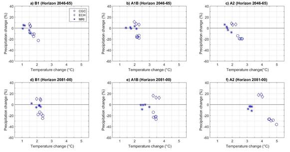
Figure 5 Climate change signals over the Tampaon River Basin as estimated by the three GCMs for the horizons 2046-2065 (upper panels) and 2081-2100 (lower panels) under the B1(a and d), A1B (b and e) and A2 (c and f) scenarios.

Results are somewhat more mixed for precipitation; from Figure 5 and Figure 6 it could be seen that, over the two basins, CGC predicts a decrease in precipitation, while ECH predicts an increase in precipitation. On the other hand, MRI shows small changes in precipitation over the two basins.
In addition, Figure 5 and Figure 6 show that the spread of the relative changes both in temperature and precipitation for the horizon 2081-2100 is larger than the spread of relative changes for the horizon 2046-65, especially for the A2 scenario. This highlights how climate model uncertainty varies when considering the prediction horizon and the emission scenario. Furthermore, it can be seen that the relative changes in precipitation and temperature obtained with the ensemble simulations can overlap the relative changes in precipitation and temperature of another GCM (e.g., horizon 2046-2065 under the B1 scenario; Figure 5a), so that the NCV uncertainty is comparable to the GCM uncertainty (in this horizon under the B1 scenario). In contrast, the uncertainty related to the NCV becomes less important in the horizon 2081-2100 (e.g.,Figure 5f). This result is in agreement with the work of Hawkins and Sutton (2009), which analyzes different sources of uncertainty in the prediction of the surface air temperature. The authors showed that the relative weight of the main sources of uncertainty in climate impact studies (i.e., emission scenario, climate model and natural climate variability) varies with the prediction lead time. Hence, the dominant sources of uncertainty are associated with climate models and emission scenarios for prediction horizons of many decades.
Uncertainty associated with natural climate variability on hydrological indicators
Figure 7 and Figure 8 show the relative changes on the selected hydrological indicators between the reference (1971-2000) and future (2046-2065) periods (as computed with Equation 6) over the Tampaon River Basin and the Papagayo River Basin, respectively.
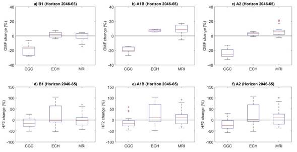
Figure 7 Relative changes (as calculated with Eq. 6) of overall mean flow (OMF, upper panels) and 2-yr return period high flow (HF2, lower panels) between the reference (1971-00) and the future (horizon 2046-65) periods over the Tampaon River Basin. The boxplots depict the median and the 25th and 75th percentiles.

From these figures it could be seen that CGC generally leads to negative relative changes on OMF; however, ECH and MRI often provide positive and negative relative change values for this indicator. For instance, over the Papagayo River Basin under the A1B scenario (Figure 8b), the simulated OMF values by ECH varies between -4.5% and +6.3%, with a median value of -0.1%. It can be noticed that, in some cases, the range of the relative differences of OMF obtained with one GCM covers the range of the relative differences obtained with another GCM. For example, over the Tampaon River Basin (A1B scenario; Figure 7b), the relative difference of OMF simulated by MRI ranges from -5.5% to 17%, and covers the relative difference of OMF obtained with ECH (between 7% and 9%); however, the median relative differences of OMF are very close between both GCMs, with OMF values of about 8%. This situation is more common for the high flow indicator (Figures 7d, 7e and 7f), indicating that the climate change signals on HF2 obtained with different GCMs may be similar due to the NCV uncertainty.
The Wilcoxon rank-sum test (Wilcoxon, 1945) is performed to assess if two samples obtained from two distinct GCMs are independent or not. The Wilcoxon test results showing the rejection or not of the null hypothesis (i.e., the two series are independent samples from identical continuous distributions with equal medians) are depicted in the following tables. Table 3 and Table 4 compares (in pairs), for a given GCM, the series of the climate change impacts on the indicators from the three emission scenarios (B1, A1B and A2) for the Tampaon River Basin and the Papagayo River Basin, respectively. Similarly, Table 5 and Table 6 compares (in pairs), for a given emission scenario, the series of the climate change impacts on the indicators from the three GCMs (CGC, ECH and MRI) for the Tampaon River Basin and the Papagayo River Basin, respectively. The gray areas in Tables 3 to 6 indicate a no rejection of the null hypothesis, that is, a similarity in the climate change signal due to the NCV.
Table 3 Wilcoxon test results (p-values) of the comparison of scenario pairs for the Tampaon River Basin. The gray areas indicate no rejection of the null hypothesis at significance level of 5%.
| CGC | ECH | MRI | ||||||||
|---|---|---|---|---|---|---|---|---|---|---|
| Ind. | Hor. | B1-A1B | B1-A2 | A1B-A2 | B1-A1B | B1-A2 | A1B-A2 | B1-A1B | B1-A2 | A1B-A2 |
| OMF | 2046- 2065 |
0.712 | 0.030 | 0.088 | 0.001 | 0.605 | <0.001 | <0.001 | <0.001 | 0.229 |
| 2081- 2100 |
<0.001 | <0.001 | 0.002 | <0.001 | <0.001 | 0.114 | 0.063 | 0.003 | 0.081 | |
| HF2 | 2046- 2065 |
0.954 | 0.222 | 0.174 | 0.796 | 0.436 | 0.863 | 0.125 | 0.222 | 0.907 |
| 2081- 2100 |
0.383 | 0.112 | 0.269 | 0.436 | 0.436 | 0.436 | 0.712 | 0.628 | 0.756 | |
Table 4 Same as table 3 but for the Papagayo River Basin.
| CGC | ECH | MRI | ||||||||
|---|---|---|---|---|---|---|---|---|---|---|
| Ind. | Hor. | B1-A1B | B1-A2 | A1B-A2 | B1-A1B | B1-A2 | A1B-A2 | B1-A1B | B1-A2 | A1B-A2 |
| OMF | 2046- 2065 |
0.4263 | 0.0436 | <0.001 | 0.077 | 0.1359 | <0.001 | 0.4263 | 0.0914 | <0.001 |
| 2081- 2100 |
0.415 | 0.017 | 0.2443 | <0.001 | 0.014 | 0.6048 | 0.4492 | 0.0298 | 0.229 | |
| HF2 | 2046- 2065 |
0.6554 | 0.8461 | 0.6414 | 0.3401 | 0.0625 | 0.004 | 0.8766 | 0.4492 | 0.4263 |
| 2081- 2100 |
0.9227 | 0.393 | 0.3825 | 0.3401 | 0.3865 | 0.9314 | 0.6695 | 0.6004 | >0.99 | |
Table 5 Wilcoxon test results (p-values) of the comparison of GCM pairs for the Tampaon River Basin. The gray areas indicate no rejection of the null hypothesis at significance level of 5%.
| CGC-ECH | CGC-MRI | ECH-MRI | ||||||||
|---|---|---|---|---|---|---|---|---|---|---|
| Ind. | Hor. | B1 | A1B | A2 | B1 | A1B | A2 | B1 | A1B | A2 |
| OMF | 2046- 2065 |
<0.001 | <0.001 | <0.001 | <0.001 | <0.001 | <0.001 | 0.258 | 0.310 | 0.118 |
| 2081- 2100 |
<0.001 | <0.001 | <0.001 | <0.001 | <0.001 | <0.001 | <0.001 | 0.532 | 0.009 | |
| HF2 | 2046- 2065 |
0.086 | 0.029 | 0.019 | 0.214 | 0.015 | 0.001 | 0.292 | 0.458 | 0.435 |
| 2081- 2100 |
0.001 | 0.001 | <0.001 | <0.001 | <0.001 | <0.001 | 0.226 | 0.086 | 0.017 | |
Table 6 Same as Table 5 but for Papagayo River Basin.
| CGC-ECH | CGC-MRI | ECH-MRI | ||||||||
|---|---|---|---|---|---|---|---|---|---|---|
| Ind. | Hor. | B1 | A1B | A2 | B1 | A1B | A2 | B1 | A1B | A2 |
| OMF | 2046- 2065 |
<0.001 | <0.001 | <0.001 | 0.005 | <0.001 | 0.756 | 0.969 | <0.001 | 0.002 |
| 2081- 2100 |
<0.001 | <0.001 | <0.001 | 0.002 | 0.074 | 0.006 | <0.001 | <0.001 | <0.001 | |
| HF2 | 2046- 2065 |
0.369 | 0.274 | 0.042 | 0.304 | 0.027 | 0.641 | 0.585 | 0.482 | 0.160 |
| 2081- 2100 |
0.032 | 0.009 | 0.067 | 0.187 | 0.214 | 0.587 | 0.585 | 0.056 | 0.051 | |
When emission scenarios are compared, the null hypothesis is not rejected in all cases for HF2 (Tables 3 and 4). Results for OMF are more mixed, since over the Tampaon River Basin for the 2081-2100 period, the null hypothesis is rejected for all cases for CGC but not for ECH and MRI (Table 3).
In addition, when GCMs are compared (Tables 5 and 6), results show a general rejection of the null hypothesis for OMF. The exception is made for the Tampaon River Basin at the 2046-2065 horizon, where the null hypothesis is not rejected for the ECH-MRI model pair in any scenario. For OMF over the Papagayo River Basin, the comparison of OMF series leads to no rejection of the null hypothesis in the three isolated cases. However, the results are different for HF2: over the Tampaon River Basin (Table 5), the null hypothesis is not rejected in most cases, when the ECH-MRI model pair is tested. Similarly for the Papagayo River Basin (Table 6), most of the CGC-MRI model pair and all the ECH-MRI model pair lead to a no rejection of the null hypothesis.
These results show a large uncertainty on the high flow indicator, but this uncertainty is more related to the NCV than to the choice of the GCM or the emission scenario. On the other hand, we can see that the NCV uncertainty is less important for OMF than for HF2.
Conclusion
The scope of this work is the evaluation of the impacts of climate change on the hydrology of two contrasted catchments in Mexico, by considering three types of uncertainty: climate model, emission scenario and Natural Climate variability (NCV).
Regarding the projected changes on meteorological variables, the analysis shows a large variability on precipitation over the two catchments, since the selected GCMs provide both an increase and a decrease in future precipitation. It is also noted that the uncertainty associated with the NCV is an important source of uncertainty depending on the emission scenario considered.
It is well described in the literature that the largest source of uncertainty in climate change impact studies on water resources is the choice of the GCM (e.g., Graham, Hagemann, Jaun, & Beniston, 2007). Accordingly, our results show that climate model uncertainty is a key factor for impact studies. However, the uncertainty associated with the NCV cannot be neglected in hydrological climate change impact studies. In the present work, the results demonstrate that the uncertainty related to the NCV is critical in the evaluation of the impacts of climate change on high flows, and to some extent, comparable to the GCM uncertainty and emission scenario uncertainty.
Future work should consider additional basins in order to explore the contrasted climate types and climate variability that determine the hydrological regimes of the Mexican territory. In addition, other sources of uncertainty should be evaluated, such as the bias correction method and the hydrological model uncertainties. Finally, the present work based on the CMIP3 multi-model dataset will be next validated according to the recent climate model simulations from the CMIP5 multi-model dataset.
Acknowledgments
We acknowledge the modeling groups, the Program for Climate Model Diagnosis and Intercomparison (PCMDI) and the WCRP's Working Group on Coupled Modelling (WGCM) for their roles in making available the WCRP CMIP3 multi-model dataset.
REFERENCES
Arnell, N. G., & Gosling, S. N. (2013). The impacts of climate change on river flow regimes at the global scale. Journal of Hydrology, 486, 351-364. [ Links ]
Arnold, J. G., Srinivasan, R., Muttiah, R. S., & Williams, J. R. (1998). Large area hydrologic modeling and assessment part I: Model development 1. JAWRA Journal of the American Water Resources Association, 34(1), 73-89. [ Links ]
Braun, M., Caya, D., Frigon, A., & Slivitzky, M. (2012). Internal variability of Canadian RCM’s hydrological variables at the basin scale in Quebec and Labrador. Journal of Hydrometeorology, 13, 443-462. [ Links ]
CICESE, Centro de Investigación Científica y de Educación Superior de Ensenada. (2017). Base de datos climatológica nacional. Ensenada, México: Centro de Investigación Científica y de Educación Superior de Ensenada. Recuperado de http://clicom-mex.cicese.mx [ Links ]
Deser, C., Knutti, R., Solomon, S., & Phillips, A. S. (2012). Communication of the role of natural variability in future North American climate.Nature Climate Change, 2(11), 775-779. [ Links ]
Githui, F., Gitau, W., Mutua, F., & Bauwens, W. (2009). Climate change impact on SWAT simulated streamflow in western Kenya. International Journal of Climatology, 29, 1823-1834. [ Links ]
Graham, L. P., Hagemann, S., Jaun, S., & Beniston, M. (2007). On interpreting hydrological change from regional climate models. Climatic Change, 81, 97-122. [ Links ]
Gratiot, N., Duvert, C., Collet, L., Vinson, D., Némery, J., & Sáenz-Romero, C. (2010). Increase in surface runoff in the central mountains of Mexico: Lessons from the past and predictive scenario for the next century. Hydrology and Earth System Sciences, 14, 291-300. DOI: 10.5194/hess-14-291-2010 [ Links ]
Hawkins, E., & Sutton, R. (2009). The potential to narrow uncertainty in regional climate predictions. Bulletin of the American Meteorological Society, 90, 1095-1107. [ Links ]
IMTA, Instituto Mexicano de Tecnología del Agua. (2018). Banco Nacional de Datos de Aguas Superficiales (BANDAS). Jiutepec, México: Instituto Mexicano de Tecnología del Agua. Recuperado de https://www.imta.gob.mx/bandas [ Links ]
IPCC, Intergovernmental Panel on Climate Change. (2010). Emissions Scenarios: IPCC Special Report. Cambridge, UK: Cambridge University Press. [ Links ]
IPCC, Intergovernmental Panel on Climate Change. (2014). Contribution of Working Group II to the Fifth Assessment Report of the Intergovernmental Panel on Climate Change: Impacts, adaptation, and vulnerability. Cambridge, UK, & New York, USA: Cambridge University Press. [ Links ]
Jung, T. (2005). Systematic errors of the atmospheric circulation in the ECMWF forecasting system. Quarterly Journal of the Royal Meteorological Society, 131, 1045-1073. DOI:10.1256/qj.04.93 [ Links ]
Maderey, L. E., Jiménez, A., & Carrillo, J. J. (2013). Global climate change and its effect on hydrological resources of Mexico’s central region. Analele stiintifice ale Universitatii "Alexandru Ioan Cuza" din Iasi-seria Geografie, 59(1), 59-78. [ Links ]
Meehl, G. A., Covey, C., Taylor, K. E., Delworth, T., Stouffer, R. J., Latif, M., McAvaney, B., & Mitchell, J. F. B. (2007). THE WCRP CMIP3 Multimodel dataset: A new era. Climate Change Research. Bulletin of the American Meteorological Society , 88, 1383-1394. [ Links ]
Mendoza, V. M., Villanueva, E. E., & Adem, J. (1997). Vulnerability of basins and watersheds in Mexico to global change. Climate Research, 9, 139-145. [ Links ]
Molina-Navarro, E., Hallack-Alegría, M., Martínez-Pérez, S., Ramírez-Hernández, J., Mungaray-Moctezuma, A., & Sastre-Merlín, A. (2016). Hydrological modeling and climate change impacts in an agricultural semiarid region. Case study: Guadalupe River Basin, Mexico.Agricultural Water Management, 175, 29-42. [ Links ]
Mpelasoka, F. S., & Chiew, F. H. S. (2009). Influence of rainfall scenario construction methods on runoff projections. Journal of Hydrometeorology , 10, 1168-1183. [ Links ]
Muerth, M. J., Gauvin St-Denis, B., Ricard, S., Velázquez, J. A., Schmid J., Minville, M., Caya, D., Chaumont, D., Ludwig, R., & Turcotte, R. (2013). On the need for bias correction in regional climate scenarios to assess climate change impacts on river runoff. Hydrology and Earth System Sciences , 17, 1189-1204. [ Links ]
Neitsch, S. L., Arnold, J. G., Kiniry, J. R., Williams, J. R., & King, K. W. (2002). Soil and water assessment tool theoretical documentation version 2000. Texas, USA: Texas Water Resources Institutes. [ Links ]
Peel, M. C., Finlayson, B. L., & McMahon, T. A. (2007). Updated world map of the Köppen-Geiger climate classification. Hydrology and Earth System Sciences , 11, 1633-1644. [ Links ]
Rivas, I., Güitrón, A., & Montero, M. (2011). Hydrologic vulnerability to climate change of the Lerma-Chapala Basin, Mexico.Sustainability Today, 297-308. [ Links ]
Robles-Morua, A., Che, D., Mayer, A. S., & Vivoni, E. R. (2015). Hydrological assessment of proposed reservoirs in the Sonora River Basin, Mexico, under historical and future climate scenarios.Hydrological Sciences Journal, 60(1), 50-66. [ Links ]
Sedue, Secretaría de Desarrollo Urbano y Ecología. (1986). Estudio de calidad y clasificación del río Tampaón, San Luis Potosí y Querétaro México, DF: Secretaría de Desarrollo Urbano y Ecología. [ Links ]
Tapia, E. M., Minjarez, I., Espinoza, I., & Minjarez, C. (2014). Use of Stella Software for the modelling of climate change impacts on water balance for the Rio Yaqui Basin, Sonora, Mexico. European Scientific Journal, ESJ, 10(14) 351-360. [ Links ]
Teutschbein, C., Wetterhall, F., & Seibert, J. (2011). Evaluation of different downscaling techniques for hydrological climate-change impact studies at the catchment scale. Climate Dynamics, 37, 2087-2105. [ Links ]
Troin, M., Velázquez, J. A., Caya, D., & Brissette, F. (2015). Comparing statistical post-processing of regional and global climate scenarios for hydrological impacts assessment: A case study of two Canadian catchments. Journal of Hydrology , 520, 268-288. [ Links ]
Velázquez, J. A., Schmid, J., Ricard, S., Muerth, M. J., Gauvin St-Denis, B., Minville, M., Chaumont, D., Caya, D., Ludwig R., & Turcotte, R. (2013). An ensemble approach to assess hydrological models’ contribution to uncertainties in the analysis of climate change impact on water resources. Hydrology and Earth System Sciences , 17, 565-578, DOI: 10.5194/hess-17-565-2013 [ Links ]
Velázquez, J. A., Troin, M., & Caya, D. (2015). Hydrological modeling of the Tampaon River in the context of climate change.Tecnología y ciencias del agua, 6(5), 17-30. [ Links ]
Velázquez-Zapata, J. A., Troin, M., & Dávila-Ortiz, R. (2017). Evaluación del impacto del cambio climático en los indicadores hidrológicos de una cuenca del centro de México con base en un ensamble de modelos climáticos y en el modelo hidrológico SWAT.Ingeniería, Investigación y Tecnología, 18(3), 341-351. [ Links ]
Received: August 31, 2018; Accepted: March 26, 2019
 Este es un artículo publicado en acceso abierto bajo una licencia Creative Commons
