Study área

The high Cauca basin is located in southwestern Colombia. The Cauca river follows a south-north direction in an inter-andean valley (Figure 1). In the first 153 km, the channel descends 2.8 km to reach Salvajina reservoir, whose drainage area is 3,652 km². Downstream, the basin reaches 5,111 km² at La Balsa station and finally the area of interest closes at the Juanchito hydrometric station, covering a total of 8,556 km². Both stations were selected considering: 1) the proximity to the reservoir outlet, 2) Juanchito station is the control point for the volume operation in the Salvajina dam and 3) Juanchito is located on the outskirts of the city of Cali, which is the third most populous city in Colombia with 2.4 million inhabitants.

Figure 1 Location of the high Cauca basin and the hydrological network (left). Monthly rainfall in the area tributary to the reservoir and the tributary flow rate to Salvajina (right and above). Monthly storage in the Salvajina reservoir and average flow rate at Juanchito regulation target station (right and below). 

The Salvajina reservoir has a maximum storage capacity of 848 hm³, its operation objectives are flood and estuarine control, guaranteeing flow rates between 900 m³ / s and 130 m³ / s for 95% of the time at Juanchito station (^{Sandoval, Ramirez, & Santacruz, 2011}).

The hydrological regime in the region is strongly affected by the climatic variability associated with the double passage of the Intertropical Convergence Zone (ITCZ), orography, the processes that occur in the Atlantic ocean, the Caribbean sea, the Pacific and the Amazon, but above all, by the influence of the ENSO phenomenon in its extreme phases (^{García, Botero, Bernal, Ardila, & Piñeros, 2012}; ^{Puertas & Carvajal, 2008}; ^{Rueda & Poveda, 2006}).

Mean annual rainfall in the upper Cauca river basin is 1900 mm, and a bimodal cycle with greater rainfall predominates in the periods: March-April-May (MAM) and September-October-November (SON) (Figure 1, right) (^{Sandoval & Ramirez, 2007}). Strong connections have been reported between mean monthly flow rates of various rivers in western Colombia with the El Niño Oceanic Index - 𝑂𝑁𝐼, and other signs of change in the surface temperature of the Pacific ocean, the Pacific Decadal Oscillation - PDO, with composite climatic signals for atmospheric and oceanic variables such as the ENSO - MEI Multivariate Index and exclusively atmospheric variables such as the Chorro del Chocó - CCC and the SOI Southern Oscillation Index, among others (^{Jiménez-Cisneros et al., 2014}; ^{Poveda, Jaramillo, & Vallejo, 2014}; ^{Poveda et al., 2006}).

Reservoir index

^{López and Francés (2013)} propose an IE reservoir index (Equation 1), which establishes the degree of alteration of the hydrological regime based on the percentage of unregulated area, and the percentage of average runoff that cannot be retained in the reservoir.

Where, ARit is the tributary area to the reservoir in km², in year t, AS is the area tributary to the station in km², CS is the mean volume drained in the basin to station S in the year t and in hm³, CR is the total storage capacity of the reservoir in hm³ in year t; and N the number of reservoirs upstream of the station. For a basin with a single reservoir at the head and without other significant anthropic changes over time (eg transfer, increase / decrease of reservoirs, etc.) that affect the variables ARit y CRit, this Index works as a discrete variable or change signal that is intense / weak depending on the proximity of the capacity station of interest to the dam, and has been used in statistical non-stationary flood modeling (^{Liang, Jing, Wang, Binquan, & Zhao, 2017}; ^{Machado et al., 2015}).

The impacts of a reservoir on the rolling of floods depends upon: the available capacity of the reservoir, the size of the works in relation to basin water supply, the uses of stored water and water levels in the reservoir before the channel, etc. (^{Moreno, Begueria, Garcés, & García, 2003}). Available capacity means the free volume or difference between the maximum storage capacity and the volume of water at any given time. Changes in available capacity may limit / favor the management of maximum annual flow rates at the target station. Therefore, in this paper it is proposed to adjust equation 1, replacing the relationship between reservoir capacity and average runoff, by the annual reserve volume coefficient D(t)=CRt-Vat/CRt) that determines the proportion of volume available versus the capacity of the reservoir, so that the index IE2 is:

Where Vat is the mean annual volume stored in the Salvajina reservoir, estimated with data from bathymetry conducted by the CVC in 1985, 2003 and 2011, and the reservoir end-of-day level records. With this change, in addition to the effect of a decrease in regulatory capacity as the tributary area at the capacity station increases (established by the ratio of areas), the index considers volume management as a condition that influences observed maximum annual flow rates.

Indices of climatic variability

Bearing in mind that the ENSO phases are defined by the US National Ocean and Atmosphere Agency (NOAA) based on the El Niño Oceanic Index (ONI), in this work the mean annual value of ONI is adopted as a criterion to classify each hydrological year, as follows: one year is considered La Niña if the ONI mean annual value ≤ -0.30; El Niño years occur when ONI ≥ 0.30; and a year is defined as Normal, provided that -0.30 < ONI < 0.30. The low frequency climatic indices used in the modeling correspond to the mean annual values of the El Niño Oceanic Index - ONI or quarterly moving mean of the anomalies of Pacific surface temperature in the Niño3-4 region and the ENSO - MEI Multivariate Index, which corresponds to the First Principal Component of a set of oceanic and atmospheric signals throughout the Tropical Pacific region. All values are estimated based on information published by ^{NOAA (2017)}.

Generalized Additive Models of Location, Scale and Shape parameters-GAMLSS

GAMLSS models assume that the response variable Y (Q_max) has a cumulative probability distribution function, whose parameters may be a function of one or more explanatory variables (climatic and reservoir indices). That is, for yt independent variables at time t=1,2,…,n; there is a function FY(yt│θt), where the parameters θt=µt, σt,υt,τt can change based on a set of m explanatory variables Xmt=x1t,x2t,…,xmt through a monotonic link function gk θk presented in Equation (3) (^{Stasinopoulos, Rigby, Vlasios, Heler, & Bastiani De, 2015}):

Where θk and ηk are vectors of length n; Xk is an array of covariates of order n x m; βk is a vector of parameters of length m; hjk(xjk) represent smoothing in the distribution parameters; and xjk is a vector of covariates for j = 1,2,…, m.

As a smoothing function, the B-splines, pb () which are polynomial parts used in additive models, are evaluated, with the advantage that they minimize the degrees of freedom (df) of the model, through different methods e.g.: Maximum Likelihood (ML), GAIC, etc. More information can be found in ^{Stasinopoulos et al. (2015)}.

Non-stationary return period

The return period T is an indicator of the rarity of flooding, that is, the average time that elapses until, for the first time, a flood exceeds a given value (yp0). It is commonly used to define the design flow rate of a hydraulic work or to reference the level of flood threat. Considering that the statistics of this event follow a geometric distribution, the probability that the first flood exceeds yq0 at time x is fx=px∏t=1x-11-pt,  x=1,2,…,xmax (^{Salas & Obeyskera, 2014}), where f1=p1 and xmax is the time at which pt becomes unity. If the probability pt is constant over time fx=PX=x=1-px-1p, therefore, the return period or Expected Wait Time (EWT) is:

Where p and q are the probability of exceedance and without exceedance, respectively. When the probability pt is non-stationary, then the return period changes over time:

The values of the probability of exceedance 𝑝 𝑡 are obtained from pt=1-FYyq0,θt using the available data. yp0 is a reference flow rate for a non-stationary Frequency Analysis model of which the parameter θt varies in accordance with the covariates Xmt (^{Obeyskera & Salas, 2016}). Considering Equation (5), in the hydraulic design and management of water resources, questions arise: What is the value of T of a historical event, associated with a non-stationary flood model? What is the design flow rate, if the value of T is variable in time? Because of this, ^{Salas and Obeyskera (2014)} propose to determine the non-stationary T value, using a non-homogeneous geometric distribution:

Where the values pt=1-qt, are obtained from pt=1-FYyq0,θt, for the preset yq0 and the non-stationary statistical model. ^{Salas Obeysekera and Vogel (2018)}, and ^{Serinaldi (2015)} present another simplified way of estimating the non-stationary return period, based on the concept of “Average Annual Risk” economic analysis (AAR) expressed as: AARn=p-=1/np1+p2+…+pn. Where it is assumed that for a period n, the risk can be described by the mean of the sequence of probabilities of exceedance (p1,p2,…,pn), due to this, non-stationary T equals:

^{Serinaldi (2015)} argues that one of the most important indicators in the planning and design of hydraulic works is the Risk of Failure 𝑅 or probability 𝑅 that an extreme event will be observed at least once yq0 during the useful life n of a works. This expression being the most appropriate or direct to define the design flow rate against an acceptable level of risk since it depends on the probability of exceedance and not on the return period. When i.i.d. conditions exist, i.i.d. R=PX≤n=FXn=∑x=1nfx=1-(1-p)n (^{Chow, Maidment, & Mays, 1994}); however, under conditions of non-stationarity ^{Salas et al. (2018)} use the concepts Expected Wait Time and Average Annual Risk to determine the risk of non-stationary failure:

Where pt and p- are the probability of exceedance and the probability of multi-year mean exceedance, respectively. Highlighting that REWT and RAAR are solved numerically.

Identification of changes and trends in the flood regime

The non-parametric statistical tests of ^{Mann-Kendall (Mann, 1945}; ^{Yue & Wang, 2002}) and ^{Pettitt (1979)} are applied to the time series to analyze the stationarity. Additionally, in order to address the effects of reservoir operation, the maximum annual flood series were divided into the periods: 1965-1984 and 1986-2015, thereby representing the unregulated regime and the altered regime, respectively.

Adjustment and selection of non-stationary statistical models

GAMLSS models are used to force gradual changes in the location parameter μ based on the ONI, MEI and IE2. covariates. The probability distribution functions selected are: Gumbel (GU), Lognormal (LN) and Gamma (GA). All have two parameters μ, σ, they are suitable to counteract the effects of positive asymmetry, common in series of hydrological extremes. The results will focus on the best models obtained and not on the set of models evaluated.

Two types of statistical models are analyzed: Stationary models (M0), where both distribution parameters are independent; and the models of external covariates (M1), in which the location parameter μ can depend linearly on one or several climatic indices, on the reservoir index or on the combination of both types of explanatory variables. The selection of the models is based on the Generalized Akaike Information Criteria (GAIC) and the Schwartz Bayesian Criteria (SBC) (Equation (10) and Equation (11)):

Where l^ = ln (ML), the maximum likelihood of the model is ML, then k: required penalty associated with the number of parameters of the distribution and df: degrees of freedom. In this work, a penalty k = 3.0 is adopted, in such a way that the degree of complexity of the model does not degrade the ability to describe the behavior of the series and conserves as much as possible the principle of parsimony.

In the absence of a statistic to determine the goodness of fit of the GAMLSS models, ^{Stasinopoulos et al. (2015)} propose to verify the normality of the residuals, for this the Filliben correlation coefficient and the behavior of the graphs without the residuals trend (worm-plot) are evaluated. This ensures that the selected model represents the systematic part and that the remaining (residual) information is white noise.

The return period in non-stationary models

To compare the results obtained in the M0 and M1 models, the EWT and AAR formulations are used. The calculation starts by defining a flow rate yp0 with the stationary model, then the non-stationary model M1 is used to estimate the probability of exceedance, equations 4 to 9 are applied to determine the hydrological risk in terms of non-stationary T and R, considering between other aspects: the moment at which pt becomes unity, the length 𝑛 of records and the predominant pattern of change in M1. It is important to mention that, for each station, R is estimated for the design flow rate of T = 100 years and different values n of working life.

Altered flood regime

Next, the changes in the flood regime in La Balsa and Juanchito are analyzed.

Table 1 confirms that the flow rate at La Balsa decreases during the registration period and this trend is significant at α=0.05. In addition, there are points of change in the mean in 1975 and 1984 that coincide with phase changes of the PDO and the commissioning of the reservoir. Due to the proximity of the station to the reservoir output it is possible to associate the non-stationarity with anthropic alteration. Figure 3b shows the decrease in the magnitude of Juanchito's floods between 1965 and 1984, but this change has no statistical significance (Table 1). On the contrary, between 1986 and 2015, a gradual and significant increase in annual maximum flow rate is observed, although this increase does not necessarily respond to a linear correlation (Figure 3b). There are also identified points of change in the mean in 1984 and the 1970s and 1990s that coincide in the first moment with the commissioning of the reservoir, and the rest with PDO phase changes, a high rate of occurrence of ENSO events (five reported in the 1970s and 1980s) (^{Wolter & Timlin, 1998}), and historical floods of the Cauca river in 1971, 1974, 1975, 1982, 1984, 1988, 1997 and 1999, 2008, 2010 and 2011 (^{Enciso et al., 2016}), that affect the mean of the time series.

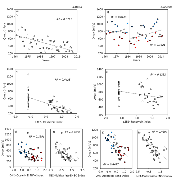
Figure 3 Variation of annual floods. From left to right La Balsa and Juanchito; a), b) time evolution; c), d) Connection with the IE2 reservoir index; e)-h) Relationship with the ONI and MEI indices, highlighted in blue and red the flow rates observed in La Niña and El Niño years, respectively. 

The following physical processes that may be related to the trends of increase in the flood regime of Juanchito station between 1986 and 2015 are:

The results obtained in Table 1 highlight the difficulty in accepting / rejecting the i.i.d. hypothesis for the 1965-2015 period at Juanchito station, since the non-parametric tests applied indicate stationarity. However, changes in the slope of the trend lines in the RN and RA periods mask the continuous increase in annual flooding in the last 30 years of the analysis period and therefore, the RA sample requires the non-stationary Flooding Frequency Analysis.

Figure 3 shows the behavior of maximum annual floods as a function of time and reservoir and climate indices, which suggest that although there is a moderate linear correlation (0.30<r<0.70), the variability explained by the selected indices is low. This is understandable, given the complex connection between flow rates and climatic variables that do not necessarily conform to linear models, therefore, it may be necessary to include smoothing functions in non-stationary statistical modeling.

Non-stationary statistical models of the flood regime in the Cauca

River

The results of the statistical modeling of the annual maximum daily flow rates for La Balsa (1965-2015) and Juanchito (1986-2015) are presented below.

Table 2 shows that the stationary model (M0) in La Balsa follows the Lognormal distribution (LN2). The Log transformation helps reducing the positive asymmetry of the observations. Then, the floods in Juanchito conform to the Gamma distribution, which is a function that has a smooth form and does not require the Log function to counteract the asymmetry; This last result is similar to that obtained by ^{Enciso et al. (2016)}, who finds that Juanchito's annual maximum daily flow rates in the 1986-2015 period are adequately adjusted to a Log Pearson III distribution, which is a generalization of the Gamma distribution. Next, it can be seen that the GAIC statistic suggests that the M1 models have lower loss of information. Regarding the quality of fit, in all cases, the Filliben correlation coefficients are higher than the critical values, therefore, the hypothesis of normality in the residuals is accepted and the models are adequately adjusted to the observations.

^{Debele, Bogdanowicz and Strupczewski (2017)} suggest that the selection of the distribution function (fdp) is one of the most important decisions for the proper analysis of the models. We consider that the hypothesis tests establish an adequate fitting, but do not necessarily lead to the selection of the best fdp. For this, GAMLSS models provide a broad range of comparison options between different families of fdp and also the consideration of non-stationarity. However, it is necessary to use the expert’s criterion to select a pfd that controls the effect of the positive asymmetry characteristic of the hydrological series and a model without over-parameterization.

Among non-stationary models with the best fit we have:

It is important to highlight that based on the evidence of non-stationarity, it is necessary to adopt methodologies that incorporate change patterns and allow a comparative analysis of results. In this work, the non-stationary models based on co-variables (M1) show a better representation of the variability of the time series, considering that the majority of the observations are within the band of quantiles 1% to 99% of the models (Figure 4a and Figure 4b). ^{Villarini, Serinaldi, Smith, & Krajewski (2009b)} obtained similar results using GAMLSS for the analysis of floods in a US basin, mentioning that the models manage to capture the wide dispersion and nonlinearity of data for percentiles between 5 and 95%.

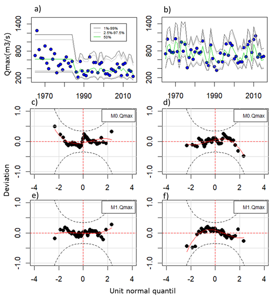
Figure 4 Statistical models. From left to right: annual floods at La Balsa and Juanchito; a) and b) the temporal variation of different percentiles in the range 1% - 99% of the M1 model (solid lines), the blue dots correspond to the observations. Theoretically, between 60% and 90% of observations are expected to be within the area covered by the 1% and 99% percentiles of the model; c)-f) contain the worm-like graphics of the residuals of the M0 and M1 models, respectively. 

The non-stationary M1 models show - for all the percentiles plotted - that at certain times the magnitude of the variables obtained is different from that estimated under stationary conditions, e.g. during La Niña years, and that increases in the magnitude of flow rates that can affect flood risk indicators such as the return period and the risk of failure for a particular project life can be identified. Regarding this result, ^{López and Francés (2014)}, when evaluating floods in the Northwest of Mexico, also find a significant influence of the ENSO phenomenon in the inter-annual variability of the flood regime, highlighting increases in magnitude during La Niña. In addition to the above, it is necessary to recognize that a limitation of the results of the co-variable models is the uncertainty associated with ignorance about the future, e.g. the behavior of the explanatory variables beyond the registration period (there are no long-term projections for the ENSO indices that may be incorporated into the predictive power of the models) and that other physical processes (not considered in the present study) may be more significant to describe the variability of floods.

Figures 4c-4f evaluate the normality of the residuals of the different models based on their configuration. In a Q-Q graph with no tendencies, which is usually shaped like a worm, one seeks for the continuous red line (trend) to be similar to a straight line, parallel and close to the horizontal axis. On the contrary, when the residuals show accentuated configurations either in S or U, they indicate high asymmetry and / or kurtosis (^{Buuren & Fredriks, 2001}). In both stations, it is evident that the models meet the normality condition. However, of all of them, the M1 model of La Balsa has fewer deviations from that assumption.

Analysis of changes in the return period

Figure 5 and Table 3 show the variations obtained when estimating the period of return T and risk of failure R, for the selected stationary and non-stationary models. Figures 5a and 5b contain the variation of non-stationary T as a function of stationary T, following the methods of Expected Wait Time (EWT) and Average Annual Risk (AAR) (^{Salas et al., 2018}). This paper establishes that the maximum annual flow rates at La Balsa have a long-term tendency to decrease, so that the probabilities of exceedance also suggest a decreasing pattern. Figure 4a establishes the variation of non-stationary 𝑇, highlighting two things: first, for 1≤T≤5 years, the non-stationary model indicates that TEWT<T. This corresponds to an increase in the probability of observing minor floods. However, when using the AAR method, no differences can be seen between non-stationary T and T≤20 years, (TAAR≅T), this situation can be associated with the fact that in the first 20 years of records (1965-1984) the hydrological series was not affected by the reservoir, so the mean of the probability of exceedance remains constant and similar to that of the stationary model. Second, from the aforementioned inflection points, it is appreciated that TEWT>T and TAAR>T, thus, the decrease in the magnitude of the floods during the altered regime (1986-2015) leads to the decrease in hydrological risk expressed as the probability of observing a flood equal to that of the reference or increase in non-stationary T. Said behavior of increase and subsequent decrease of the hydrological risk can be seen directly in Figure 4c where the risk of failure R associated with a T=100 years flood flow rate or the probability of observing, at least once, a flood equal to that of the reference in a period of 𝑛 years of working life. In the case of La Balsa, a REWT,AAR larger than the stationary is observed for works with n<20 years and a lower risk, from 30 years of working life. Another aspect to note is that the non-stationary 𝑅 values in each station are identical regardless of the method of determination, so their use could be a more direct way of establishing the design flow rate of a hydraulic works for a predefined acceptable level of risk.

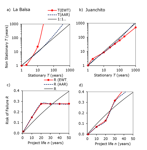
Figure 5 Variation of the Return Period and Risk of Failure of the statistical models of La Balsa (left) and Juanchito (right). Above, evolution of non-stationary T as a function of stationary T. Below, changes in risk as function of working life. 

In the case of annual floods at Juanchito between 1986 and 2015, an increasing trend has been described (Figure 3b). When comparing the non-stationary return period, Figure 5b shows: 1) When 1<T<7 years TEWT>T and TAAR>T are obtained. Therefore, the co-variable model indicates that the most frequent floods have a lower probability of occurrence in comparison with the stationary model. After seven years, the opposite occurs: TEWT<T and TAAR<T. Although graphically this difference is modest, the decrease of TEWT against T ranges between 14% and 50%, whereas between TAAR and T varies between 15% and 39%, with a slight increase when T is 1,000 years. Among the possible explanations for the evolution of TAAR are the gentle slope of change of the annual maximum flow rates, its significance (α=0.10) and the short length of the time series (30 years). In any case, the information obtained highlights a slight increase in the probability of occurrence of extreme maximum floods. Which leads us to consider that although the management of the reservoir has positive effects on the most common floods, there are external factors (climatic variability, increase in precipitation, changes in the unregulated basin, etc.) that negatively affect the objective of regulation of the rarest and most extreme floods. Similar information is presented in Figure 5d, in which case REWT, AAR<T for a working life of n≤ 25 years, but from said n, the risk failure of the non-stationary model exceeds that of the stationary R.

All the changes in the hydrological risk indicators (Qmax, T y R), are of interest for flood management at Juanchito, not only because this is the target station for volume control in the Salvajina reservoir; but because the unplanned urban growth in the city of Cali, as in many other cities in developing countries, has led to intensive building developments in the flood plains of both banks of the Cauca River. About 900 thousand inhabitants of the city are located in a flood risk area on the right bank of the Cauca river. Flood control is managed through the operation of the reservoir and lateral levees built for a T=30 year flood. Despite these structures, the changes in the hydrological risk identified are corroborated by historical flow rates observed in 2008, 2010, 2011 and 2017; and more than ten floods in the Juanchito area recorded in the last decade (^{El País, 2011}; ^{Enciso et al., 2016}), highlighting the need to provide for a natural disaster risk management program that incorporates a systemic view of the problems and includes change patterns associated with climate variability.

REFERENCES

Ahn, K., & Palmer, R. (2016). Use of a nonstationary copula to predict future bivariate low flow frequency in the Connecticut River basin. Hydrological Processes, 30(19), 3518-3532. Recuperado de https://doi.org/10.1002/hyp.10876 [ Links ]
Ávila, Á., Guerrero, F., Escobar, Y., & Justino, F. (2019). Recent precipitation trends and floods in the Colombian Andes. Water, 11(2), 379. Recuperado de https://doi.org/10.3390/w11020379 [ Links ]
Banco Mundial. (2014). Notas de política Colombia: hacia la paz sostenible, la erradicación de la pobreza y la prosperidad compartida. Washington, DC, EUA: Banco Mundial. Recuperado de http://www.bancomundial.org/content/dam/Worldbank/Feature Story/lac/Colombia Policy Notes pub SPA 11-7-14web.pdf [ Links ]
Buuren, S. V., & Fredriks, M. (2001). Worm plot: A simple diagnostic device for modelling growth reference curves. Statistics in Medicine, 20(8), 1259-1277. Recuperado de https://doi.org/10.1002/sim.746 [ Links ]
Carvajal, Y., Jiménez, H., & Materon, H. (1998). Incidencia del fenómeno ENSO en la hidroclimatología del valle del río Cauca-Colombia. Bull. l'Institut Français d'Études Andines, 27(3). Recuperado de http://www.redalyc.org/resumen.oa?id=12627336 [ Links ]
Chow, V. T., Maidment, D. R., & Mays, L. W. (1994). En: Suarez, M. (ed.). Hidrología aplicada, 2ª ed. Bogotá, Colombia: McGraw-Hill. [ Links ]
Córdoba, S., Palomino, R., Gámiz, S., Castro, Y., & Esteban, M. (2015). Influence of tropical Pacific SST on seasonal precipitation in Colombia: Prediction using El Niño and El Niño Modoki. Climate Dynamics, 44(5-6), 1293-1310. Recuperado de https://doi.org/10.1007/s00382-014-2232-3 [ Links ]
Debele, S. E., Bogdanowicz, E., & Strupczewski, W. G. (2017). Around and about an application of the GAMLSS package to non-stationary flood frequency analysis. Acta Geophysica, 65(4), 885-892. Recuperado de https://doi.org/10.1007/s11600-017-0072-3 [ Links ]
El País. (2011). Conozca el drama de los habitantes de Juanchito causado por las inundaciones. El País. Recuperado de https://www.elpais.com.co/cali/conozca-el-drama-de-los-habitantes-de-juanchito-causado-por-las-inundaciones.html [ Links ]
EM-DAT. (2018). The emergency events database - Universite Catholique de Louvain (UCL)-. Brussels, Belgium: CRED, D. Guha-Sapir. Recuperado de www.emdat.be [ Links ]
Enciso, A., Carvajal, Y., & Sandoval, M. (2016). Hydrological analysis of historical floods in the upper valley of Cauca River. Ingeniería y Competitividad, 57(1), 46-57. [ Links ]
Escalante-Sandoval, C., & Garcia-Espinoza, E. (2014). Analysis of annual flood peak records in Mexico. WIT Transactions on Information and Communication Technologies, 47, 49-60. Recuperado de https://doi.org/10.2495/RISK140051 [ Links ]
García, M., Botero, A., Bernal, F., Ardila, E., & Piñeros, A. (2012). Variabilidad climática, cambio climático y el recurso hídrico en Colombia. Revista de Ingeniería. Universidad de los Andes, 36(0121-4993), 60-64. Recuperado de http://ojsrevistaing.uniandes.edu.co/ojs/index.php/revista/article/view/136 [ Links ]
Garreaud, R., Vuille, M., Compagnucci, R., & Marengo, J. (2009). Present-day South American climate. Palaeogeography, Palaeoclimatology, Palaeoecology, 281(3-4), 180-195. Recuperado de https://doi.org/10.1016/j.palaeo.2007.10.032 [ Links ]
Gutiérrez, F., & Dracup, J. (2001). The use of ENSO based streamflow forecasts for reservoir operations in Colombia. In: Bridging the gap (pp. 1-7). Reston, USA: American Society of Civil Engineers. Recuperado de https://doi.org/10.1061/40569(2001)164 [ Links ]
Herzog, S. K., Martinez, R., Jorgensen, P., & Tiessen, H. (eds.). (2012). Cambio climático y biodiversidad en los Andes tropicales. París, Francia: Instituto Interamericano para la Investigación del Cambio Global (IAI), São José dos Campos, y Comité Científico sobre los Problemas del Medio Ambiente (SCOPE). [ Links ]
IDEAM-PNUD-MADS-DNP-Cancillería, Instituto de Hidrología, Meteorología y Estudios Ambientales, Programa de las Naciones Unidas para el Desarrollo, Ministerio de Ambiente y Desarrollo Sostenible, Departamento Nacional de Planeación, & Cancillería. (2015). Nuevos escenarios de cambio climático para Colombia 2011-2100: tercera comunicación nacional de cambio climático. Recuperado de http://modelos.ideam.gov.co/media/dynamic/escenarios/documento-nacional-departamental-2015.pdf [ Links ]
Jiménez-Cisneros, B. E., Oki, T., Arnell, N. W., Benito, G., Cogley, J. G., Döll, P., Jiang, T., & Mwakalila, S. S. (2014). Freshwater resources. In: Field, C. B., Barros, V. R., Dokken, D. J., Mach, K. J., Mastrandrea, M. D., Bilir, T. E., Chatterjee, M., Ebi, K. L., Estrada, Y. O., Genova, R. C., Girma, B., Kissel, E. S., Levy, A. N., MacCracken, S., Mastrandrea, P. R., & White, L. L. (eds.). Climate change 2014: Impacts, adaptation, and vulnerability. Part A: Global and sectoral aspects (pp. 229-269). Cambridge, UK, New York, USA: Cambridge University Press, Working Group II to the Fifth Assessment Report of the Intergovernmental Panel on Climate Change. [ Links ]
JMA & WMO, Japan Meteorological Agency & World Meteorological Organization. (2017). El Nino monitoring and outlook/TCC. Recuperado de http://ds.data.jma.go.jp/tcc/tcc/products/elnino/decadal/pdo.html [ Links ]
Khaliq, M. N., Ouarda, T. B. M. J., Ondo, J. C., Gachon, P., & Bobée, B. (2006). Frequency analysis of a sequence of dependent and/or non-stationary hydro-meteorological observations: A review. Journal of Hydrology, 329(3-4), 534-552. Recuperado de https://doi.org/10.1016/j.jhydrol.2006.03.004 [ Links ]
Liang, Z., Jing, H. Y., Wang, Y., Binquan, L., & Zhao, J. (2017). A sample reconstruction method based on a modified reservoir index for flood frequency analysis of non-stationary hydrological series. Stochastic Environmental Research and Risk Assessment, 32. Recuperado de https://doi.org/10.1007/s00477-017-1465-1 [ Links ]
Lima, C., & Lall, U. (2011). Spatio-temporal non-stationary flood frequency modeling: seasonal peak floods in southern Brazil modeled using pre- and concurrent Pacific and Atlantic Ocean conditions. AGU Fall Meeting Abstracts, 1, 06. Recuperado de http://adsabs.harvard.edu/abs/2011AGUFM.H24C.06L [ Links ]
López de la, J., & Francés, F. (2013). Non-stationary flood frequency analysis in continental Spanish rivers, using climate and reservoir indices as external covariates. Hydrology and Earth System Sciences, 17(8), 3189-3203. Recuperado de https://doi.org/10.5194/hess-17-3189-2013 [ Links ]
López de la, J., & Francés, F. (2014). La variabilidad climática de baja frecuencia en la modelación no estacionaria de los regímenes de las crecidas en las regiones hidrológicas Sinaloa y Presidio San Pedro. Tecnología y ciencias del agua, 5(4), 79-101. Recuperado de http://www.redalyc.org/pdf/3535/353532522005.pdf [ Links ]
Machado, M., Botero, B., López de la, J., Francés, F., Díez, A., & Benito, G. (2015). Flood frequency analysis of historical flood data under stationary and non-stationary modelling. Hydrology and Earth System Sciences, 19(6), 2561-2576. Recuperado de https://doi.org/10.5194/hess-19-2561-2015 [ Links ]
Mann, H. (1945). Non-parametric tests against trend. Econométrica, 13(3), 163-171. Recuperado de https://doi.org/10.2307/1907187 [ Links ]
Matalas, N. C. (1997). Stochastic hydrology in the context of climate change. Climatic Change, 37, 89-101. [ Links ]
Méndez, J., Ramírez, A., Cornejo, E., Zárate, A., & Cavazos, T. (2011). Teleconexiones de la oscilación decadal del Pacífico (PDO) a la precipitación y temperatura en México. Investigaciones Geográficas, (73). Recuperado de http://www.scielo.org.mx/scielo.php?script=sci_arttext&pid=S0188-46112010000300005 [ Links ]
Milly, P. C. D., Betancourt, J., Falkenmark, M., Hirsch, R. M., Kundzewicz, Z. W., Lettenmaier, D. P., Stouffer, R. J., Dettinger, M. D., & Krysanova, V. (2015). On critiques of “Stationarity is dead: Whither water management?” Water Resources Research, 51(9), 7785-7789. Recuperado de https://doi.org/10.1002/2015WR017408 [ Links ]
Milly, P., Betancourt, J., Falkenmark, M., Hirsch, R., Kundzewicz, Z., Lettenmaier, D., & Stouffer, R. (2008). Stationarity is dead: Whither water management ? Science, 319(February), 573-574. [ Links ]
Montanari, A., & Koutsoyiannis, D. (2014). Modeling and mitigating natural hazards: Stationarity is immortal! Water Resources Research, 50(12), 9748-9756. Recuperado de https://doi.org/10.1002/2014WR016092. [ Links ]
Moreno, J., Begueria, S., Garcés, L., & García, J. (2003). Intensidad de las avenidas y aterramiento de embalses en el Pirineo Central español. Ería, (61), 159-167. Recuperado de https://doi.org/10.17811/ER.0.2003.159-167 [ Links ]
NOAA-ESRL-PSD, National Oceanic and Atmospheric Administration, Earth System Research Laboratory, & Physical Sciences Division. (2017). Climate indices: monthly atmospheric and ocean time series. Recuperado de https://www.esrl.noaa.gov/psd/data/climateindices/list/ [ Links ]
NOAA, National Oceanic and Atmospheric Administration. (2017). Pacific Decadal Oscillation (PDO)-Northwest Fisheries Science Center. Recuperado de https://www.nwfsc.noaa.gov/research/divisions/fe/estuarine/oeip/ca-pdo.cfm [ Links ]
Obeyskera, J., & Salas, J. D. (2016). Frequency of recurrent extremes under non-stationarity. Journal of Hydrologic Engineering, 21(5), 04016005. Recuperado de https://doi.org/10.1061/(ASCE)HE.1943-5584.0001339 [ Links ]
Pettitt, A. N. N. (1979). A non-parametric approach to the change-point problem. Applied Statistics, 28(2), 126-135. Recuperado de https://doi.org/10.2307/2346729 [ Links ]
Poveda, G. (2004). La hidroclimatología de Colombia: Una síntesis desde la escala interdecadal. Revista de la Academia Colombiana de Ciencias Exactas, Físicas y Naturales, 28-107, 201-222. Recuperado de http://www.clas.ufl.edu/users/prwaylen/geo3280articles/Synthesis of Colombian hydrology.pdf [ Links ]
Poveda, G., & Álvarez, D. (2012). El colapso de la hipótesis de estacionariedad por cambio y variabilidad climática: implicaciones para el diseño hidrológico en ingeniería. Revista de Ingeniería. Universidad de los Andes, 36(0121-4993), 65-76. [ Links ]
Poveda, G., Jaramillo, L., & Vallejo, L. (2014). Seasonal precipitation patterns along pathways of South American low-level jets and aerial rivers. Water Resources Research, 50(1), 98-118. Recuperado de https://doi.org/10.1002/2013WR014087 [ Links ]
Poveda, G., Velez, J., Mesa, O., Hoyos, C., Mejía, F., Barco, O., & Correa, P. (2002). Influencia de fenómenos macroclimáticos sobre el ciclo anual de la hidrología colombiana: cuantificación lineal, no lineal y percentiles probabilísticos. Meteorología Colombiana, (6), 121-130. Recuperado de http://www.geociencias.unal.edu.co/unciencias/data-file/user_23/file/METEOROLOGIA/13Poveda Clima Nuevo.pdf [ Links ]
Poveda, G., Waylen, P., & Pulwarty, R. (2006). Annual and inter-annual variability of the present climate in northern South America and southern Mesoamerica. Palaeogeography, Palaeoclimatology, Palaeoecology, 234(1), 3-27. Recuperado de https://doi.org/10.1016/j.palaeo.2005.10.031 [ Links ]
Puertas, O., & Carvajal, Y. (2008). Incidencia de El Niño-Oscilación del Sur en la precipitación y la temperatura del aire en Colombia, utilizando el Climate Explorer. Revista Científica Ingeniería y Desarrollo, (23), 104-118. Recuperado de http://rcientificas.uninorte.edu.co/index.php/ingenieria/article/view/2097/1346 [ Links ]
Rigby, R. A., & Stasinopoulos, M. (2005). Generalized additive models for location, scale and shape. Journal of the Royal Statistical, 54, Part3(3), 507-554. Recuperado de https://doi.org/10.1111/j.1467-9876.2005.00510.x [ Links ]
Rueda, O., & Poveda, G. (2006). Variabilidad espacial y temporal del Chorro del Chocó y su efecto en la hidroclimatología de la región del Pacífico colombiano. Meteorología Colombiana, (501), 132-145. [ Links ]
Salas, J. D., Obeysekera, J., & Vogel, R. M. (2018). Techniques for assessing water infrastructure for nonstationary extreme events: A review. Hydrological Sciences Journal, 63(3), 325-352. Recuperado de https://doi.org/10.1080/02626667.2018.1426858 [ Links ]
Salas, J. D., & Obeyskera, J. (2014). Revisiting the concepts of return period and risk for nonstationary hydrologic extreme events. Journal of Hydrologic Engineering, 19(3), 554-568. Recuperado de https://doi.org/10.1061/(ASCE)HE.1943-5584.0000820 [ Links ]
Sandoval, M., & Ramirez, C. (eds.). (2007). El río Cauca en su valle alto: un aporte al conocimiento de uno de los ríos más importantes de Colombia. Cali, Colombia: CVC, Corporación Autónoma Regional del Valle del Cauca. Recuperado de http://www.cvc.gov.co/index.php/servicio-al-ciudadano/inscriba-departamento-de-gestion-ambiental/77-recurso-hidrico/1386-libro-rio-cauca [ Links ]
Sandoval, M., Ramirez, C., & Santacruz, S. (2011). Optimización de la regla mensual de operación del embalse de Salvajina. Ingeniería de Recursos Naturales y del Ambiente, (6), 93-104. Recuperado de http://bibliotecadigital.univalle.edu.co/handle/10893/2596 [ Links ]
Serinaldi, F. (2015). Dismissing return periods! Stochastic Environmental Research and Risk Assessment, 29(4), 1179-1189. Recuperado de https://doi.org/10.1007/s00477-014-0916-1 [ Links ]
Stasinopoulos, M., Rigby, R. A., Vlasios, V., Heler, G., & Bastiani De, F. (2015). Flexible regression and smoothing the GAMLSS packages in R. Recuperado de http://www.gamlss.org/wp-content/uploads/2015/07/FlexibleRegressionAndSmoothingDraft-1.pdf [ Links ]
Vasiliades, L., Galiatsatou, P., & Loukas, A. (2015). Nonstationary frequency analysis of annual maximum rainfall using climate covariates. Water Resources Management, 29(2), 339-358. Recuperado de https://doi.org/10.1007/s11269-014-0761-5 [ Links ]
Villarini, G., Smith, J., Serinaldi, F., Ntelekos, A., & Schwarz, U. (2012). Analyses of extreme flooding in Austria over the period 1951-2006. International Journal of Climatology, 32(8), 1178-1192. Recuperado de https://doi.org/10.1002/joc.2331 [ Links ]
Villarini, G., & Strong, A. (2014). Roles of climate and agricultural practices in discharge changes in an agricultural watershed in Iowa. Agriculture, Ecosystems & Environment, 188, 204-211. Recuperado de https://doi.org/10.1016/j.agee.2014.02.036 [ Links ]
Villarini, G, Smith, J. A., Serinaldi, F., Bales, J., Bates, P. D., & Krajewski, W. F. (2009a). Flood frequency analysis for nonstationary annual peak records in an urban drainage basin. Advances in Water Resources, 32(8), 1255-1266. Recuperado de https://doi.org/10.1016/j.advwatres.2009.05.003 [ Links ]
Villarini, G., Serinaldi, F., Smith, J. A., & Krajewski, W. F. (2009b). On the stationarity of annual flood peaks in the continental United States during the 20th century. Water Resources Research, 45(8), 1-17. Recuperado de https://doi.org/10.1029/2008WR007645 [ Links ]
Wang, S., Huang, J., He, Y., & Guan, Y. (2015). Combined effects of the Pacific decadal oscillation and El Niño-Southern Oscillation on global land dry-wet changes. Scientific Reports, 4(6651). Recuperado de https://doi.org/10.1038/srep06651 [ Links ]
Wolter, K., & Timlin, M. (1998). Measuring the strength of ENSO events: How does 1997/98 rank? Weather, 53(9), 315-324. Recuperado de https://doi.org/10.1002/j.1477-8696.1998.tb06408.x [ Links ]
Yue, S., & Wang, C. Y. (2002). Applicability of prewhitening to eliminate the influence of serial correlation on the Mann-Kendall test. Water Resources Research, 38(6), 4-1. Recuperado de https://doi.org/10.1029/2001WR000861 [ Links ]
Received: September 26, 2018; Accepted: August 23, 2019
Este es un artículo publicado en acceso abierto bajo una licencia
Creative Commons