


 texto en
  Artículo en XML
 Referencias del artículo
 Enviar artículo por email
 Citado por SciELO
  Similares en
SciELO
Similares en
SciELO 
 Permalink
Introduction
In the design of irrigation canals and the modeling of hydrodynamic runoff in channels, empirical relationships are used to estimate the friction, for example: Chezy’s resistance factor, Manning’s roughness coefficient or the Darcy-Weisbach friction factor (Wu, Shen, & Chou, 1999). By contrast, in fluid mechanics where the movements of the particles in a flow field are described, the condition close to the wall is an unknown that must be included as a boundary (Panton, 2013). Therefore, a way to describe the average flow field is through a hypothesis, in which, at the bottom, the particles have no slip and the outer field away from the wall follows a pattern similar to that used in the empirical relationships.
The development of the velocity profile is a function of the fluid’s properties, such as viscosity (Schlichting & Gersten, 2017). In the case of flow in a canal or natural channel, the law of shear stress for the laminar sublayer considering a Newtonian fluid is represented as follows:
where τ is the shear stress, μ the dynamic
viscosity, y the vertical coordinate and
For the case of the outer region and different flow conditions (mainly the turbulent one), the shear stress is not constant, since it is proportional to the variation in the average velocity with respect to the vertical coordinate (Schlichting & Gersten, 2017). From this, Prandtl introduced the parameter of shear velocity (u * ) in the hydraulic field to represent the shear stress of the entire section, this by means of an expression that relates the shear stress at the wall (τ 0 ) and the fluid density (ρ) (Equation 2) (Keulegan, 1938).
In the outer region of the velocity field of a turbulent flow, the value of the shear
stress maintains its influence, even when the local gradient of the profiles is zero (
In studies made in rough-bottomed ducts, it has been observed that turbulence production energy is immediate to the bottom and greater than in the case of smooth bottoms. This is due to the diameter of the bottom particle, which, due to being big offers greater resistance to fluid movement, generates a higher friction stress (Cebeci & Chang, 1978; Coleman & Alonso, 1983; Zanoun, Durst, & Nagib, 2003). Therefore, the shear model is related to the deformation of the velocity profile and the roughness of the wall.
Due to the characteristics represented by the shear velocity in a turbulent flow, it has been applied in diverse subjects such as: empirical model approach to mean velocity and turbulence intensity distribution (George, 2007; Nezu & Nakagawa, 1993), sediment transport (Celestini, Silvagni, Spizzirri, & Volpi, 2007; van Rijn, 1984), scouring and characterization of roughness in articulated hydraulic concrete mats for the protection of channels. In more recent years, it has been applied in the study and characterization of turbulent flows with the dimensionless relationship approach in turbulent correlation models (Auel, Albayrak, & Boes, 2014; Motlagh & Taghizadeh, 2016; Qiao, Delavan, Nokes, & Plew, 2016).
According to the literature review, different methods have been used to estimate shear velocity; however, the procedure is not explicitly indicated and only the theoretical basis of determination is presented (Auel et al., 2014). For this reason, the aim of this work was to present a methodology that allows experimentally determining shear velocity, considering the log-law as a model of velocity distribution in the outer region of turbulent flow.
Materials and methods
von Kármán’s mean velocity distribution model
Different models to represent velocity distribution in an open channel flow are found in the literature (Spalding, 1961); however, in the practice of hydraulic engineering, the most widely used model is that of von Kármán, which has three conditions. The first is to represent the viscous or laminar sublayer where the turbulent stresses have no influence and the viscous forces (v) dominate (Equation 3).
The second represents the transition zone, also called the buffer zone, where the turbulent and viscous stresses are of the same order (Shih, Povinelli, Liu, Potapczuk, & Lumley, 1999) (Equation 4).
The third considers the outer zone or turbulent region where the viscous stresses have no influence (Equation 5). This condition is known as the log-law (George, 2007).
The log-law has two empirical variables: the von Kármán constant (κ) and the additive constant (A). According to Zanoun et al. (2003), the values of 0.4 for κ and 5.5 for A, parameters used in practice for an open channel flow, are considered adequate (Equation 6).
Each of the equations comprising the von Kármán model has a validity range as a function of the parameter yu * /v and indicates the evaluation zone of the three flow regions: viscous, transition and outer sublayer.
Shear velocity estimation
For the experimental study it is important to know the boundaries of the outer
region (Equation 6). According to
the experimental results of Tominaga and Nezu
(1992), the point closest to the bottom in mean velocity flows in the
vertical
Equation 6 uses the estimate of
the averaged flow velocity
In order to process the experimental data, the velocity measurement pertaining to
the outer zone was assessed to discard the points outside the range of analysis.
Subsequently, the shear value was estimated with the instantaneous velocity (
The subscript
Equation 7 is not explicit since the shear velocity is found on both sides of the expression; therefore, for its solution, the fixed-point algorithm described by Burden and Faires (2011) was applied.
According to Schmid and Lazos-Martínez (2000), in the measurement of a random variable, the results generally follow, in good approximation, a normal distribution. In the case of flow velocity, there are results that validate this hypothesis to a certain degree. This subject is widely discussed by Frisch (1995) and Davidson (2004); however, in this case, the probability density function (PDF) of the data obtained by evaluating Equation 7 is unknown. Therefore, the final value representative of the shear velocity u * was calculated with the median of the u *i,j values obtained.
Anderson-Darling test of the shear model
As part of the data analysis, the Anderson-Darling normality test was performed to determine if the data follow a normal distribution, this by calculating the statistical value of the test (Equation 8).
According to Stephens (1974), the critical value is 0.754 for a significance level of 5 % and when the number of data (n) is greater than 100. Therefore, if the statistical value A 2 , of the test for the sample, is less than 0.754, it is accepted that the data follow a normal distribution; otherwise, the possibility that the data follow a central tendency distribution is rejected.
Due to the fact the PDF was unknown, and in order to ensure 50 % coverage of the data around the representative value of u * , the location of the first (Q 1 ) and third (Q 3 ) quartile of the data ordered in increasing form was calculated (Equations 9 and 10, respectively).
From the location of the first and third quartiles the u *i,j values were located and the interquartile range was obtained.
Experimental station
The tests were carried out in the variable slope experimental channel at the Hydraulic Laboratory of the Mexican Institute of Water Technology (IMTA, for its Spanish acronym); the channel has a smooth, metallic, rectangular-shaped bottom with a 0.245-m-wide base and 5 m long (Figure 1). The experimental station has a 10-hp pump that supplies the flow, a measuring weir calibrated with ISO standard 1438 (International Organization for Standardization, 2008), and a valve to regulate the flow, among other components that allow for stable experimental conditions.

For measuring the instantaneous velocities, the Nortek® Vectrino Profiler™ ADV device was used; it allows sampling the three velocity components in a profile of up to 30 mm, with a separation of 1 mm between cells and with a sampling frequency of 1-100 Hz. The device was positioned 3.5 m away from the flow inlet to avoid defects in the velocity profile caused by the inflow of the flow or by its outflow in free fall to the recirculation tank.
The channel slope was slightly modified with a mechanical jack, taking care that the experimental conditions complied with the criteria of repeatability and reproducibility. The Froude (F r ) and Reynolds (R e ) numbers were calculated with Equations 11 and 12, respectively.
All the tests were done in a subcritical regime, as indicated by the Froude number values in Table 1 (F r < 1). In addition, the flow was considered fully developed turbulent, with the Reynolds number values being sufficiently high and far from the transition range (R e > 1.2 x 10⁴).
Table 1 Experimental conditions to determine the shear velocity of an open channel flow.
| Case | Slope(S, mm -1 x 10 -4 ) | Flow depth (h, cm) | Aspect ratio (b/h, mm-1) | Mean velocity ( |
Froude number (Fr) | Reynolds number (Re , x 104) |
|---|---|---|---|---|---|---|
| P-01 | 1.06 | 7.42 | 3.30 | 60.65 | 0.71 | 2.80 |
| P-02 | 1.06 | 9.80 | 2.50 | 73.06 | 0.75 | 4.01 |
| P-03 | 1.06 | 11.34 | 2.16 | 71.65 | 0.67 | 4.22 |
| P-04 | 1.06 | 12.55 | 1.95 | 84.51 | 0.76 | 5.24 |
| P-05 | 4.25 | 12.53 | 1.96 | 84.65 | 0.76 | 5.24 |
| P-06 | 4.25 | 11.16 | 2.20 | 75.84 | 0.72 | 4.43 |
| P-07 | 4.25 | 9.60 | 2.55 | 72.46 | 0.74 | 3.90 |
| P-08 | 4.25 | 7.74 | 3.17 | 57.15 | 0.65 | 2.71 |
| P-09 | 2.12 | 8.14 | 3.01 | 55.29 | 0.62 | 2.70 |
| P-10 | 2.12 | 9.03 | 2.71 | 59.86 | 0.64 | 3.11 |
| P-11 | 2.12 | 10.90 | 2.25 | 70.53 | 0.68 | 4.07 |
| P-12 | 2.12 | 12.55 | 1.95 | 81.42 | 0.73 | 5.05 |
| P-13 | 6.38 | 12.42 | 1.97 | 86.99 | 0.79 | 5.36 |
| P-14 | 6.38 | 11.26 | 2.18 | 76.18 | 0.72 | 4.47 |
| P-15 | 6.38 | 9.69 | 2.53 | 68.70 | 0.70 | 3.72 |
| P-16 | 6.38 | 7.61 | 3.22 | 57.12 | 0.66 | 2.68 |
For all tests, the measurement of the instantaneous velocities was carried out in a 12-mm profile, as close as possible to the wall, with a frequency of 100 Hz and a sampling time of 30 s.
Results and discussion
Tests
Figure 2 shows the results of a sampling of the instantaneous velocity with F r = 0.67 and R e = 4.22 x 10⁴ for cell five at 8.6 mm depth.
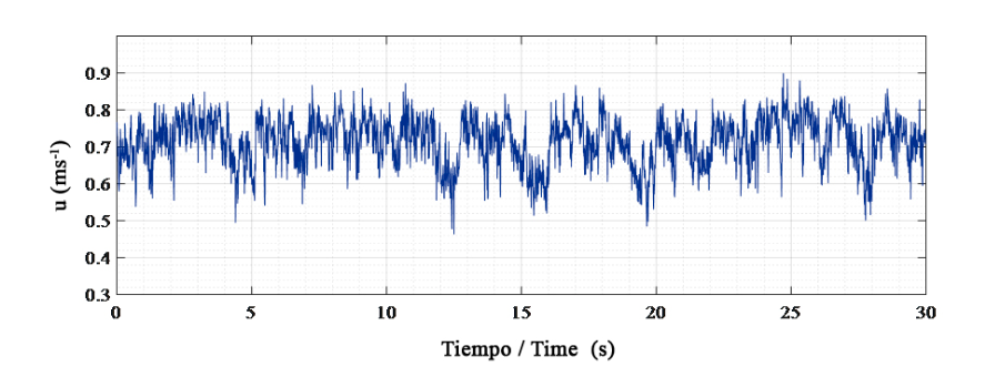
Figure 2 Record of instantaneous velocity (u) (main
direction,
The tests were conducted under the experimental conditions shown in Table 1.
The results of the processing of the experimental data are presented in Table 2, where the statistical value obtained from the Anderson-Darling test with a 5 % degree of significance and the shear velocity obtained with the model of Equation 7 are indicated.
Table 2 Results of the shear velocity and Anderson-Darling statistical value at 5 %.
| Case | Shear velocity (u* , cm-1) | Values of the interquartile range (Q1 - Q3 , cm-1) | Anderson-Darling statistical value (A2 ) |
|---|---|---|---|
| P-01 | 3.06 | 2.85 - 3.23 | 157.14 |
| P-02 | 3.55 | 3.31 - 3.76 | 14.57 |
| P-03 | 3.62 | 3.37 - 3.84 | 251.64 |
| P-04 | 4.04 | 3.81 - 4.25 | 74.92 |
| P-05 | 4.08 | 3.82 - 4.29 | 124.22 |
| P-06 | 3.73 | 3.47 - 3.96 | 881.34 |
| P-07 | 3.47 | 3.24 - 3.69 | 1.33 |
| P-08 | 2.96 | 2.76 - 3.14 | 42.43 |
| P-09 | 3.00 | 2.80 - 3.17 | 279.14 |
| P-10 | 3.15 | 2.94 - 3.33 | 184.24 |
| P-11 | 3.55 | 3.30 - 3.78 | 13.29 |
| P-12 | 3.95 | 3.71 - 4.16 | 48.31 |
| P-13 | 4.16 | 3.93 - 4.37 | 104.93 |
| P-14 | 3.76 | 3.53 - 3.97 | 19.82 |
| P-15 | 3.52 | 3.31 - 3.72 | 13.05 |
| P-16 | 3.01 | 2.79 - 3.20 | 43.40 |
The statistical values of the Anderson-Darling test (Table 2) corroborate that the PDF of the data
u
*i,j
does not follow a central tendency, since in all cases A
2
> 0.754; therefore, it is correct to represent the shear velocity
value
Figure 3 shows four dimensionless profiles drawn from the estimation of the shear velocity with a different bottom slope. It can be seen that the von Kármán model represents, with good approximation, the experimental values in their averaged condition.

In the profiles of tests P-01, P-05 and P-09, a sampling point is observed in the transition zone; this case was discarded from the data analysis since the logarithmic flow model is only for the outer region.
Conclusions
The methodology presented shows low uncertainty in the estimation of shear velocity, which can be observed in the results of the logarithmic velocity profiles. The model is also presented explicitly to obtain the shear velocity value. The Anderson-Darling test showed that the results, when evaluating the instantaneous velocity, do not follow a normal distribution, so the median is the statistical parameter to define the shear velocity value.
The application of the methodology can be extended to the use of low-frequency sampling or conventional instruments, for example a Prandtl tube, a current meter and even acoustic Doppler current profilers mounted on a mobile boat or anchored at the bottom of the channel.

