


Servicios Personalizados
Revista
Articulo
 texto en
  Artículo en XML
 Referencias del artículo
 Enviar artículo por email
Indicadores
-
 Citado por SciELO
 -
 Accesos
Links relacionados
-
 Similares en
SciELO
Similares en
SciELO
Compartir

 Permalink
Textual: análisis del medio rural latinoamericano
versión On-line ISSN 2395-9177versión impresa ISSN 0185-9439
Textual anál. medio rural latinoam. no.72 Chapingo jul./dic. 2018
https://doi.org/10.5154/r.textual.2017.72.008
Economics and public policies
The impact of interest and exchange rates on Mexican agricultural exports: a study for the period 1993-2017
1Universidad Autónoma Metropolitana, Departamento de Economía. Ciudad de México.
2Universidad Nacional Autónoma de México, Programa de Economía en la Facultad de Estudios Superiores, Acatlán, avenida Alcanfores y San Juan Totoltepe s/n, Sta Cruz Acatlán, C. P. 53150 Naucalpan de Juárez, Méx.
The objective of this paper is to determine the relationship pattern between agricultural exports and exchange and interest rates for the Mexican economy through multiple regression analysis and the Granger causality test. With the NAFTA renegotiations underway, this research seeks to contribute to the debate surrounding this treaty by presenting some of its economic results.
Keywords: Exports; agricultural sector; NAFTA; exchange rate; interest rate
El objetivo del artículo es determinar el patrón de relación entre exportaciones agrícolas, tipo de cambio y tasa de interés para la economía mexicana por medio del análisis de regresión múltiple y con la prueba de causalidad en el sentido de Granger. Ya que, en la coyuntura de la renegociación del TLCAN, esta investigación busca contribuir al debate presentando algunas aristas de los resultados económicos de dicho tratado.
Palabras clave: Exportaciones; sector agrícola; TLCAN; tipo de cambio; tasa de interés
Introduction
In 2017, the Mexican government began renegotiating the North American Free Trade Agreement (NAFTA) with the U.S. government because the latter argued that the trade deal is injurious to its economic growth.
NAFTA came into force in 1994 and established an economic policy agenda based on the idea of the free market as a mechanism to promote the internal and external competitiveness of factors of production (Puyana & Romero, 2008). However, in Mexico, the neoliberal model has failed to balance income distribution and has deepened the deficit situation in the agricultural sector.
In fact, from the signing of NAFTA until 2006, Mexico doubled its grain imports (Concheiro-Bórquez, Tarrio-García, & Grajales-Ventura, 2007) to the detriment of its food sovereignty and security (Tarrío, 2008). The panorama maintains the deficit trajectory in the main staple foods that explain a food dependence (Table 1); in the year 2000 about 5 million tons of yellow corn were imported, whereas in 2017 the volume forecast for the 2017-2018 harvest is 16.8 million tons (CNPAMM, 2017).
Table 1 Mexico. National production of main staple foods in 2016 (tons).
| Product | National production | Imports | Exports | Trade balance |
|---|---|---|---|---|
| Corn (not fodder) | 28,251 | 13,954,811 | 1,654,255 | -12,300,556 |
| Beans | 1,089 | 163,974 | 36,659 | -127,315 |
| Wheat | 3,863 | 4,646,783 | 1,543,254 | -3,103,529 |
| Soybeans | 509 | 4,038,860 | 38 | -4,038,822 |
| Poultry | 3,078 | 498,962 | 774 | -498,188 |
| Pork | 1,376 | 754,450 | 105,076 | -649,374 |
| Egg | 2,770 | 28,483 | 185 | -28,298 |
Source: author-made based on SAGARPA data
Corn for Mexico is a primordial food, which is an apparently inconsequential is- sue in terms of public policies, given that productivity in the rainfed crop from the beginning of the FTA until 2016 remained almost stagnant, in contrast to the irrigation zones -Sinaloa and Chihuahua- where there was an increase of 144 % between 1980 and 2005 (Schwentesius-Rindermann, Márquez-Berber, Almaguer-Vargas, Ayala-Garay, & Kalil Gardezi, 2006). Currently, the symmetries persist given that the yield per hectare in rainfed land is around 2 tons per hectare, while in irrigated land it is 8 tons (FIRA, 2016).
This treaty has also had an impact on the adoption of new internal food habits and problems, as asserted by Loría and Salas (2014) who cite statistical evidence indicating an increase in the proportion of spending on sweets and treats; this is part of an epidemic of excess weight and obesity along with the importation of yellow corn to supply industries related to fried foods and snacks (Moreno, 2014), impacting equally on the high levels of obesity1. This sample of diverse effects reflects a situation contrary to the objectives set out in the trade agreement, since it was established that it should contribute to the harmonious development of world trade, by reducing trade distortions and barriers in the region (NAFTA, 1994).
This paper seeks to explain the relationship pattern between agricultural exports, the exchange rate and the interest rate. Although it is generally assumed that the first variable directly impacts the external sector, a direct relationship does not fully operate in the study period between the exchange rate and exports or it is marginal, and while it is also assumed that in the free market the investment in tradable goods is largely determined by the second variable, the impact on the exportable part of the product is not entirely clear.
Despite claims to the contrary, NAFTA has perpetuated the deficit situation in the sector and in the main foods of the Mexican diet: corn and beans.
This paper is organized into three sections: the first one summarizes studies on the problems of the agricultural sector, the second presents empirical evidence about the sector and the third details the methodological proposal to estimate the relationship between agricultural exports and monetary and trade policy instruments, in addition to presenting the econometric results.
The context
In the phase preceding the FTA and during the transition to its full implementation, in an analysis of the agricultural sector in the period 1991-2000, Mella and Mercado (2006) find that the agricultural trade balance has a deficit due to higher import than export growth, with the exception of 1991 and 1995. This is contradictory since one of NAFTA’s objectives was to consolidate a favorable trade advantage, as well as to improve access to capital and technology (Crawford, 2011).
In the same sense, Lira (2014) studies the influence of the exchange rate and trade policy on agricultural exports in the period 1980-2014 by means of a VAR model, concluding that there is no statistical relationship between the variables due to the heterogeneity of the agricultural sector and its constant deficit balance. In addition, the model yields a negative sign between the proxy variable of trade openness and exports, that is, exports do not increase their competitiveness due to this single measure.
Under the scenario of the 2008-2009 crisis, Basurto and Escalante (2012) detected in these years that both imports and exports decrease; however, the deficit persists because the absolute value of the former is higher than that of the latter.
In analyzing the agricultural sector’s behavior, Puyana and Romero (2008) find that the effects of the discriminatory mechanisms of import substitution and land concentration are the determinants of the lag in the sector, since 60 % of the landowners possess less than five hectares of land and only 15 % of the land. These conditions are not expected to have changed substantially since then. In addition, Calva (2004) previously stressed the underlying structural problem in the purported integration of the three economies involved in NAFTA, that is, that the negative results in the agricultural sector observed up to 2001 were due to profound asymmetries in resources and efforts (technology, productivity and agricultural policies) between Mexico, the US and Canada. Finally, the main aspect for Mexico in this subject area is the agricultural sector’s growing deficit.
Empirical evidence
Graph 1 analyzes the behavior of the balance of agricultural and industrial products, which shows that imports grow more than exports over the period, except for the months of March in the years 2015, 2016 and 2017.
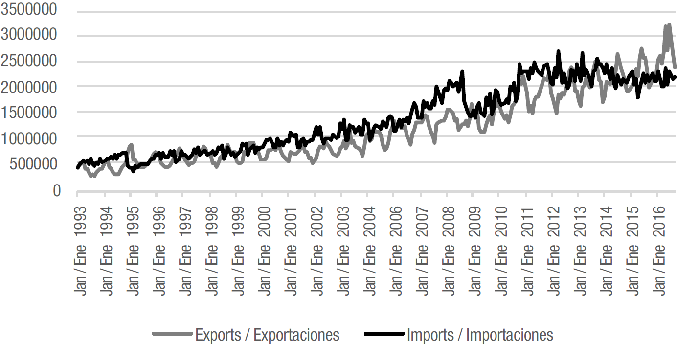
Source: author-madebased on Bank of Mexico data
Graph 1 . Balance of Mexican agricultural and industrial products 1993-2017.
While Graph 2 distinguishes the same pattern as the previous graph, imports are greater than exports when only the balance of agricultural products is considered.
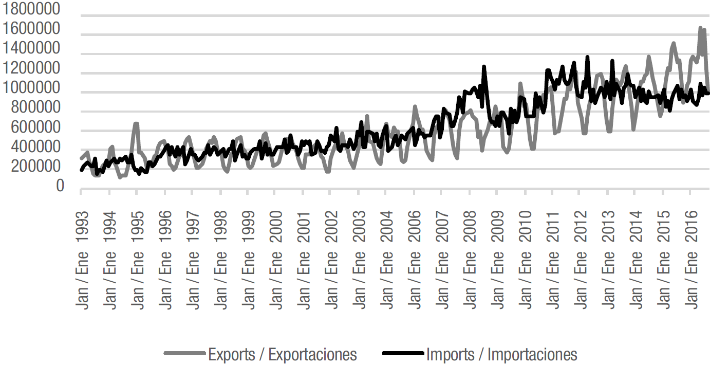
Source: author-madebased on Bank of Mexico data
Graph 2. Balance of Mexican agricultural products 1993-2017.
In addition, within the agricultural products balance, basic grains such as corn, beans and wheat have the least dynamics. In fact, Graph 3 shows that the three basic grains have maintained a persistent deficit throughout the study period.

Methodological proposal
The previous section analyzed the agricultural sector’s deficit situation and, in the search for the determinants of exports, a regression is proposed to demonstrate that, contrary to what was established, there is no evident relationship between the exchange rate and exports during the study period; the expected sign would be positive under the Marshall-Lerner condition as exports rise in the face of a devaluation (Cermeño & Rivera, 2016).
On the other hand, a negative sign is expected between exports and the interest rate2 (Ávila, J., Caamal I. and Martínez, D. (2013) , since this reduces exports (Berumen & Arriaza, 2006) and increases imports, which deteriorates the trade balance (Nadal, 2001); a study provides empirical evidence (Norton, 2004) showing agricultural activity is more sensitive to interest rate changes than other sectors.
In Graph 4, export behavior shows a growing trend throughout the period. In addition, the trend line was incorporated and this confirms the growth path of the analyzed variable.

As for the regression’s independent variables -interest rate and exchange rate- Graph 5 shows that the former has a declining trend and since 2010 its behavior has stabilized with an average of 3.82 %.
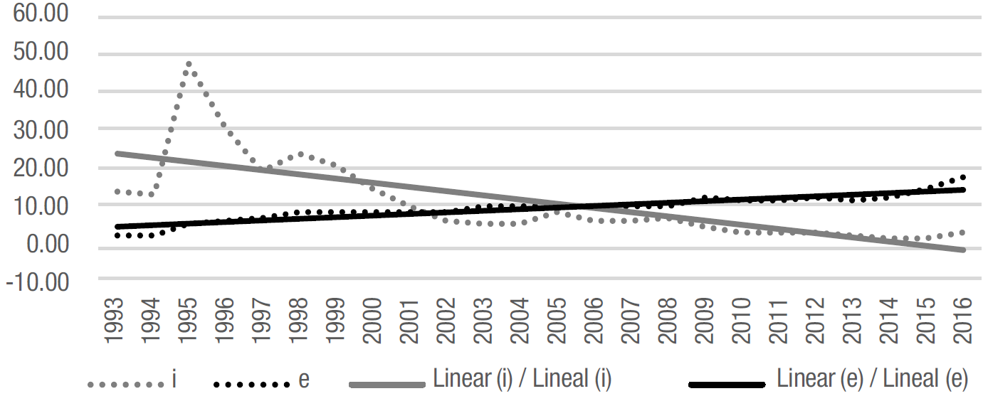
Source: author-madebased on Bank of Mexico data
Graph 5. Interest rate and exchange rate / Mexico (1993-2016).
On the other hand, the exchange rate has a smooth positive trend line, that is, the key price in trade policy has depreciated since 1993 and this is recognized by the monetary authority as a significant change for 2016 (Banxico, 2017), which is reflected in the agricultural sector’s surplus (Graph 6). This behavior also occurs in 2017, but cannot yet be classified as a structural change because it is a short period; therefore, the official position that grades the country as a power in agrofood production and export would have to be qualified (Sagarpa, 2018).
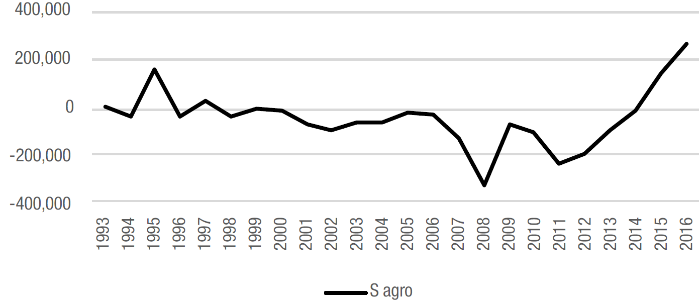
Source: author-madebased on Bank of Mexico data
Graph 6. Agricultural sector balance / México (1993-2016).
In fact, the Great Recession had a major role in the exchange rate rise and the monetary authorities took actions to smooth out the economic cycle. In Mexico, the 2008 devaluation had a positive impact of only a few months on the balance of agricultural exports (Lira, 2014), although the agricultural trade balance remained in deficit because in 2012 and 2013 there was a contraction in agricultural exports (Basurto & Escalante, 2012).
The 1994-1995 devaluation also increased exports and reduced imports (Puyana & Romero, 2008; Puyana & Romero, 2009), but the deficit trend in the agricultural trade balance in recent years stands out as the first great lie in the promises of the Treaty’s promoters (Concheiro et al., 2007), that is, it did not resolve the deficit situation in the sector.
Therefore, the three scenarios present a common denominator: a devaluation stimulates exports and depresses imports, but with a short-lived effect and does not correct the deficit situation in the agricultural sector.
Therefore, a regression was estimated for the period 1993m1-2017m7 with the Or dinary Least Squares (OLS) method; where exports (X) are based on the exchange rate (e) and the interest rate (i):
The OLS econometric technique is an a priori approach and consists of fitting the best straight line when minimizing the sum of the squared deviations of the graph points from the straight-line points (Pindyck & Rubinfeld, 2001). This technique is employed since it is an easy-to-use method and has desirable theoretical properties (Stock & Watson, 2012) for the purpose of the present research.
Basic diagnostic tests are applied to the regression to verify the quality of the estimate, based on Gujarati and Porter (2010) , which involve determining that the residuals are distributed as normal, have homocedastic variance and show no serial correlation problems.
The a posteriori approach is also used; the causality test is determined in the sense of Granger (1969) , since the existence of a correlation between two variables does not imply causality. Thus, if a lagged variable is correlated with future values of another variable, it is said that it causes or there is a correspondence relationship according to the Granger test.
The data used in this research come from the Bank of Mexico and are monthly and real, with 2008 being the base year. Considering that exports are derived from the balance of agricultural products (X), the interest rate of the 28-day CETES (Mexican federal treasury bills) was taken as a proxy variable (i) and the exchange rate is the peso to US dollar ratio (e). All three variables are expressed as an index.
Table 2 shows the first econometric exercise in which the interest rate coefficient is not significant, the exchange rate explains 37 % of agricultural exports and the model residuals exhibit problems of serial correlation and heteroscedasticity; therefore, the regression was fitted by means of Weight- ed Least Squares (WLS) and with the Cochrane-Orcutt (CO) method, with the first instrument yielding more consistent results.
Table 2 Model of agricultural exports.
| [OLS with data for the period 1993m1 to 2017m7] |
| X=91.82858+1.00000e 2.34003 (0.07494) |
| Meaning of the variables: |
| X: agricultural exports in levels. |
| e: exchange rate in levels. |
| Figures in parentheses below the coefficients represent standard errors. |
| Statistical and diagnostic tests: |
| Adjusted R2 = 0.378 |
| JB test for normality (Probability) = 0.0915 |
| Durbin-Watson = 2.2e-16 |
| Breusch-Godfrey serial correlation LM test (Probability) = 2.2e-16 |
| Breusch-Pagan test foe heteroskedasticity (Probability) = 8.12e-08 |
In the second regression the variables explain the model by 58.66%, the coeffi cients of the interest rate and the exchange rate are significant and the expected signs are verified (Table 3). The results make sense in the economic context: exports lower their level when the interest rate increases and as the exchange rate increases, on average, exports increase.
Table 3 Model of agricultural exports.
| [WLS with data for the period 1993m1 to 2017m7] |
| X=117.105462−0.142202i+0.875956e 1.440813 0.007457 (0.163354) |
| Meaning of the variables: |
| X: agricultural exports in levels. |
| i: interest rate in levels. |
| e: exchange rate in levels. |
| Figures in parentheses below the coefficients represent standard errors. |
| Statistical and diagnostic tests: |
| Adjusted R2 = 0.5866 |
| JB test for normality (Probability) = 0.001 |
| Breusch-Godfrey serial correlation LM test (Probability) = 2.2e-16 |
| Breusch-Pagan test foe heteroskedasticity (Probability) = 6.465e-06 |
However, the problems of heterocedasticity and serial correlation persist, added to which the errors are now not distributed as normal. Therefore, the structural econo metric approach does not fit the data and is limited to being able to estimate results without bias or inefficiencies in the estimators. Thus, the use of the time series ap proach is proposed, using the same variables in growth rates.
In order to determine the integration order of the series, the ADF test in its three versions (A without constant and trend, B with constant and C with trend) and the Phillips Perron test were performed. Table 4 indicates that the series can be characterized as processes without stochastic or unit root trend.
Table 4 Unit root tests.
| Phillips Perron test | |||||
|---|---|---|---|---|---|
| Variable | Value | Probability | |||
| X | -11.447 | 0.01 | |||
| I | -13.894 | 0.01 | |||
| E | -12.95 | 0.01 | |||
| ADF test | |||||
| Variable | Term | Value | Critical value | ||
| 1 % | 5 % | 10 % | |||
| X | A | -11.7753 | -2.58 | -1.95 | -1.62 |
| B | -11.8719 | -3.44 | -2.87 | -2.57 | |
| C | -11.8542 | -3.98 | -3.42 | -3.13 | |
| i | A | -13.9328 | -2.58 | -1.95 | -1.62 |
| B | -12.8692 | -3.44 | -2.87 | -2.57 | |
| C | -12.9705 | -3.98 | -3.42 | -3.13 | |
| E | A | -12.5837 | -2.58 | -1.95 | -1.62 |
| B | -12.8692 | -3.44 | -2.87 | -2.57 | |
| C | -12.9705 | -3.98 | -3.42 | -3.13 | |
When the time series are stationary, the Granger causality test is then performed.
Table 5 shows the results and in both cases the evidence suggests that the interest rate (after 9 lags) and the exchange rate (up to 8 lags) do not cause agricultural exports; in other words, exports have not been affected by variations in the exchange rate or by the monetary policy of Mexico in the period 1993-2017; their behavior is due to other determinants.
Table 5 Causality test.
| Granger test | ||||
| Null hypothesis: | i does not cause X | e does not cause X | ||
| Lag | F | Prob. | F | Prob. |
| 1 | 0.8507 | 0.3571 | 0.9029 | 0.3428 |
| 2 | 0.5826 | 0.5591 | 0.5162 | 0.5973 |
| 3 | 0.5747 | 0.6321 | 1.1128 | 0.3442 |
| 4 | 0.6778 | 0.6078 | 2.0689 | 0.08504 |
| 5 | 0.5439 | 0.743 | 1.5261 | 0.1817 |
| 6 | 0.7007 | 0.6493 | 1.7166 | 0.1171 |
| 7 | 0.8162 | 0.5745 | 1.7894 | 0.08938 |
| 8 | 1.2222 | 0.286 | 1.6039 | 0.1236 |
| 9 | 1.5458 | 0.132 | 2.0003 | 0.0395 |
| 10 | 2.5912 | 0.005 | 2.1641 | 0.02034 |
Therefore, if there is no relationship between the analyzed variables, the monetary and exchange rate policy has no impact on the trade deficit or, in other words, the efforts of the Mexican government amount to a zero-sum game.
The economic policy proposal must revolve around the US model where capitalization processes are generated (Schwentesius et al., 2006) to improve the competitiveness of rural production units.
Conclusions
After estimating the two econometric approaches and performing the relevant tests, the signs expected by economic theory were obtained in the regression. However, the diagnostic tests are not consistent and, consequently, neither are the conclusions derived.
Secondly, the Granger causality test yields statistical evidence that denies the relationship between exports and the monetary policy and exchange rate policy control variables.
These results are no more than a reflection of the agricultural sector’s structural problems, which are manifested in a deficit throughout the study period. There are years in which the devaluation of the exchange rate corrects the balance situation, but it has a short-lived effect and it has not reversed the dependency on basic products from abroad, as in the case of corn and beans.
REFERENCES
Ávila, J., Caamal, I., & Martínez, D. (2013). “El impacto de la tasa de interés y el tipo de cambio en el sector agrícola”. Revista Problemas del Desarrollo, vol. 34, núm. 135, pp. 87-104. [ Links ]
Banxico (2017). “Programa monetario” [en línea]. Recuperado el 24 de enero de 2018 de Recuperado el 24 de enero de 2018 de http://www.banxico.org.mx/publicaciones-y-discursos/publicaciones/informes-periodicos/politica-monetaria-prog-anual/%7BEF2C0392-CEC2-9F34-3DD4-D9E4A7B163FD%7D.pdf [ Links ]
Basurto, S., & Escalante, R. (2012). “Impacto de la crisis en el sector agropecuario en México”. Revista Economía UNAM, vol. 9, núm. 25, pp. 51-73. [ Links ]
Berumen, S., & Arriaza, K. (2006). “El posible impacto por el incremento de las tasas de interés en Estados Unidos sobre la economía de Guatemala”. Revista Estudios Económicos de Desarrollo Internacional, vol. 6, núm. 1, pp. 85-100. [ Links ]
Calva, J. (2004). “Ajuste estructural y TLCAN: efectos en la agricultura mexicana y reflexiones sobre el ALCA”. Revista El Cotidiano, vol. 19, núm. 124, pp. 14-22. [ Links ]
Cermeño, R., & Rivera, H. (2016). “La demanda de importaciones y exportaciones de México en la era del TLCAN. Un enfoque de cointegración”. Revista El Trimestre Económico, vol. 83, núm. 329, pp. 127-147. [ Links ]
CNPAMM (2017). “Importaciones mexicanas de maíz amarillo crecerán al menos 20% en 2017” [en línea]. El Financiero, sección economía. Recuperado el 23 de enero de 2018 de Recuperado el 23 de enero de 2018 de http://www.elfinanciero.com.mx/economia/importaciones-mexicanas-de-maiz-creceran-al-menos-20-en-2017.html [ Links ]
Concheiro-Bórquez, Tarrio-García, & Grajales-Ventura, 2007. “El TLCAN al filo de la navaja: notas para una propuesta de renegociación”. Revista Estudios Sociales y Humanisticos, vol. 5, núm. 2, pp. 108-128. [ Links ]
Crawford, T. (2011). “Impacto del TLCAN en el comercio agrícola”. Revista Mexicana de Agronegocios, vol. 15, núm. 28. pp. 457-468. [ Links ]
FIRA (2016). “Panorama Agroalimentario. Maíz 2016” [en línea]. Recuperado el 15 de enero de 2018 de Recuperado el 15 de enero de 2018 de https://www.gob.mx/cms/uploads/attachment/file/200637/Panora-ma_Agroalimentario_Ma_z_2016.pdf [ Links ]
Granger, C. (1969). “Investigating Causal Relations by Econometric Models and Cross-Spectral Methods”. Revista Econometrica, vol. 37, núm 3, pp. 424-438. [ Links ]
Gujarati, D., & Porter, D. (2010). Econometría. México: McGraw Hill. [ Links ]
Lira, R. (2014). El sector agroexportador mexicano y el tipo de cambio real 1980-2014. Elaboración de un modelo VAR. Tesis de Maestría. Benemérita Universidad Autónoma de Puebla. [ Links ]
Loría, E., & Salas, E. (2014). “Sobrepeso e integración económica en México”. Revista Economía Informa, vol. NA, núm. 389, pp. 3-18. [ Links ]
Mella, J., & Mercado, A. (2006). “La economía agropecuaria mexicana y el TLCAN”. Revista de Comercio Exterior, vol. 56, núm. 3, pp. 181-193. [ Links ]
Moreno, I. (2014). Dependencia de México a las importaciones de maíz en la era del TLCAN. Tesis de Maestría. Colegio de la Frontera Norte. [ Links ]
Nadal, A. (2001). “Lineamientos de una estrategia alternativa de desarrollo para el sector agrícola”. El Colegio de México, documento de trabajo núm. 1-05. [ Links ]
Norton, R. (2004). Política de desarrollo agrícola. Conceptos y principios. Roma: Organización de las Naciones Unidas para la Agricultura y la Alimentación. [ Links ]
Pindyck, R., & Rubinfeld, D. (2001). Econometría: modelos y pronósticos. México: McGraw Hill. [ Links ]
Puyana, A., & Romero, J. (2008). El sector agropecuario mexicano bajo el Tratado de Libre Comercio de América del Norte. La pobreza y la desigualdad se intensifican, crece la migración. En Barba, C. Retos para la integración social de los pobres en América Latina. México: CLACS- Consejo Latinoamericano de Ciencias Sociales. [ Links ]
Puyana, A. , & Romero, J. (2009). “El estancamiento del sector agropecuario mexicano”. Revista Textual, vol. NA, núm. 53, pp. 29-62. [ Links ]
SAGARPA (2018). “Prevé SAGARPA crecimiento en producción agropecuaria por más de 2.6 millones de toneladas” [en línea]. Recuperado el 24 de enero de 2018 de Recuperado el 24 de enero de 2018 de https://www.gob.mx/sagarpa/prensa/preve-sagarpa-crecimiento-en-produccion-agropecuaria-por-mas-de-2-6-millones-de-toneladas-144047 [ Links ]
Schwentesius-Rindermann, Márquez-Berber, Almaguer-Vargas, Ayala-Garay, & Kalil Gardezi, (2006). “La globalización y su efecto en la producción agrícola de las zonas áridas y semiáridas de México”. Revista Chapingo, vol. NA, núm. 5, pp. 107-116. [ Links ]
Stock, J., & Watson, M. (2012). Introducción a la econometría. Madrid: Pearson Educación. [ Links ]
Tarrío, M. (2008). “La agricultura mexicana ante el TLCAN, antecedentes, realidades y perspectivas. Un balance crítico”. Revista Textual, vol. NA, núm. 52, pp. 1-32. [ Links ]
TLCAN (2014). “Tratado de Libre Comercio de América del Norte” [en línea]. Recuperado el 23 de enero de 2018 de Recuperado el 23 de enero de 2018 de http://www.wipo.int/edocs/trtdocs/es/nafta/trt_nafta.pdf [ Links ]
Urquía, N. (2014). “La seguridad alimentaria en México”. Revista Salud Pública de México, Revista Salud Pública de México, vol. 56, núm. 1, pp. 92-98. [ Links ]
1By 2012, a quarter of the Mexican population had poor access to food, 14 % of preschool students were of short stature for their age and overweight, and obesity in children, adolescents and adults had become a public health problem (Urquía, 2014).
2In its avío (working capital) component. This rate is charged on credit granted for manufacturing or processing activities and is intended to cover the immediate needs of the business, such as financing raw materials, so as not to lose the continuity of the production cycle. The components of the interest rate - avío and refaccionario (fixed asset) - have a differentiated behavior; for the purposes of this research, only the correlation with the first is of interest, since the avío component operates negatively on investment and, therefore, on production; exports are also affected by the fall in tradable goods, that is, the quantity of goods that can be traded inside and outside a country decreases.
APPENDIX
The econometric results and the application of the tests were carried out using the computational statistical package R, version 3.3.2
First regression via OLS
Call: lm(formula = x3 ~ e3)
Residuals:
Min 1Q Median 3Q Max
-84.535 -17.852 0.659 23.305 116.483
Coefficients:
Estimate Std. Error t value Pr(>|t|)
(Intercept) 91.82858 2.34003 39.24 <2e-16 ***
e3 1.00000 0.07494 13.34 <2e-16 ***
---
Signif. codes: 0 ‘***’ 0.001 ‘**’ 0.01 ‘*’ 0.05 ‘.’ 0.1 ‘ ’ 1
Residual standard error: 40.19 on 293 degrees of freedom
Multiple R-squared: 0.378, Adjusted R-squared: 0.3758
F-statistic: 178 on 1 and 293 DF, p-value: < 2.2e-16
Diagnostic tests of the first regression via OLS
Jarque-Bera test for normality
data: e3, JB = 4.5931, p-value = 0.0915
Durbin-Watson test
data: reg4, DW = 0.0080745, p-value < 2.2e-16
alternative hypothesis: true autocorrelation is greater than 0
Breusch-Godfrey test for serial correlation of order up to 1
data: reg4, LM test = 288.28, df = 1, p-value < 2.2e-16
Studentized Breusch-Pagan test
data: reg4, BP = 28.777, df = 1, p-value = 8.12e-08
Second regression vía WLS
Call: lm(formula = x3 ~ i3 + e3, weights = pond)
Weighted Residuals:
Min 1Q Median 3Q Max
-11.9273 -1.0792 -0.3125 0.4357 11.2369
Coefficients:
Estimate Std. Error t value Pr(>|t|)
(Intercept) 117.105462 1.440813 81.277 < 2e-16 ***
i3 -0.142202 0.007457 -19.070 < 2e-16 ***
e3 0.875956 0.163354 5.362 1.67e-07 ***
---
Signif. codes: 0 ‘***’ 0.001 ‘**’ 0.01 ‘*’ 0.05 ‘.’ 0.1 ‘ ’ 1
Residual standard error: 2.788 on 292 degrees of freedom
Multiple R-squared: 0.5866, Adjusted R-squared: 0.5838
F-statistic: 207.2 on 2 and 292 DF, p-value: < 2.2e-16
Diagnostic tests of the second regression via WLS
Jarque-Bera test for normality
data: e2, JB = 27.421, p-value = 0.001
Breusch-Godfrey test for serial correlation of order up to 1
data: regp, LM test = 273.31, df = 1, p-value < 2.2e-16
Studentized Breusch-Pagan test
data: regp, BP = 23.898, df = 2, p-value = 6.465e-06
| Prueba de casualidad de Granger | |
|---|---|
| (iax) | (eax) |
| Model 1: tx ~ Lags(tx, 1:1) + Lags(ti,1:1) Model 2: tx ~ Lags(tx, 1:1) Res.Df Df F Pr(>F) 1 290 2 291 -1 0.8507 0.3571 | Model 1: tx ~ Lags(tx, 1:1) + Lags(ti,1:1) Model 2: tx ~ Lags(tx, 1:1) Res.Df Df F Pr(>F) 1 290 2 291 -1 0.8507 0.3571 |
| Model 1: tx ~ Lags(tx, 1:2) + Lags(ti,1:2) Model 2: tx ~ Lags(tx, 1:2) Res.Df Df F Pr(>F) 1 287 2 289 -2 0.5826 0.5591 | Model 1: tx ~ Lags(tx, 1:2) + Lags(ti,1:2) Model 2: tx ~ Lags(tx, 1:2) Res.Df Df F Pr(>F) 1 287 2 289 -2 0.5826 0.5591 |
| Model 1: tx ~ Lags(tx, 1:3) + Lags(ti,1:3) Model 2: tx ~ Lags(tx, 1:3) Res.Df Df F Pr(>F) 1 284 2 287 -3 0.5747 0.6321 | Model 1: tx ~ Lags(tx, 1:3) + Lags(ti,1:3) Model 2: tx ~ Lags(tx, 1:3) Res.Df Df F Pr(>F) 1 284 2 287 -3 0.5747 0.6321 |
| Model 1: tx ~ Lags(tx, 1:4) + Lags(ti,1:4) Model 2: tx ~ Lags(tx, 1:4) Res.Df Df F Pr(>F) 1 281 2 285 -4 0.6778 0.6078 | Model 1: tx ~ Lags(tx, 1:4) + Lags(ti,1:4) Model 2: tx ~ Lags(tx, 1:4) Res.Df Df F Pr(>F) 1 281 2 285 -4 0.6778 0.6078 |
| Model 1: tx ~ Lags(tx, 1:5) + Lags(ti,1:5) Model 2: tx ~ Lags(tx, 1:5) Res.Df Df F Pr(>F) 1 278 2 283 -5 0.5439 0.743 | Model 1: tx ~ Lags(tx, 1:5) + Lags(ti,1:5) Model 2: tx ~ Lags(tx, 1:5) Res.Df Df F Pr(>F) 1 278 2 283 -5 0.5439 0.743 |
| Model 1: tx ~ Lags(tx, 1:6) + Lags(ti,1:6) Model 2: tx ~ Lags(tx, 1:6) Res.Df Df F Pr(>F) 1 275 2 281 -6 0.7007 0.6493 | Model 1: tx ~ Lags(tx, 1:6) + Lags(ti,1:6) Model 2: tx ~ Lags(tx, 1:6) Res.Df Df F Pr(>F) 1 275 2 281 -6 0.7007 0.6493 |
| Model 1: tx ~ Lags(tx, 1:7) + Lags(ti,1:7) Model 2: tx ~ Lags(tx, 1:7) Res.Df Df F Pr(>F) 1 272 2 279 -7 0.8162 0.5745 | Model 1: tx ~ Lags(tx, 1:7) + Lags(ti,1:7) Model 2: tx ~ Lags(tx, 1:7) Res.Df Df F Pr(>F) 1 272 2 279 -7 0.8162 0.5745 |
| Model 1: tx ~ Lags(tx, 1:8) + Lags(ti,1:8) Model 2: tx ~ Lags(tx, 1:8) Res.Df Df F Pr(>F) 1 269 2 277 -8 1.2222 0.286 | Model 1: tx ~ Lags(tx, 1:8) + Lags(ti,1:8) Model 2: tx ~ Lags(tx, 1:8) Res.Df Df F Pr(>F) 1 269 2 277 -8 1.2222 0.286 |
| Model 1: tx ~ Lags(tx, 1:9) + Lags(ti,1:9) Model 2: tx ~ Lags(tx, 1:9) Res.Df Df F Pr(>F) 1 266 2 275 -9 1.5458 0.132 | Model 1: tx ~ Lags(tx, 1:9) + Lags(ti,1:9) Model 2: tx ~ Lags(tx, 1:9) Res.Df Df F Pr(>F) 1 266 2 275 -9 1.5458 0.132 |
| Model 1: tx~ Lags(tx,1:10)+Lags(ti,1:10) Model 2: tx ~ Lags(tx, 1:10) Res.Df Df F Pr(>F) 1 263 2 273 -10 2.5912 0.005187 | Model 1: tx~ Lags(tx,1:10)+Lags(ti,1:10) Model 2: tx ~ Lags(tx, 1:10) Res.Df Df F Pr(>F) 1 263 2 273 -10 2.5912 0.005187 |
Table 6 Mexico. Absolute data on agricultural exports (X), the interest rate (I) and the exchange rate (E).
| YEAR | X | I | E | YEAR | X | I | E | YEAR | X | I | E |
| 1993/01 | 47.6 | 217.64 | 27.94 | 2001/04 | 71.26 | 194.73 | 84.02 | 2009/07 | 66.18 | 59.75 | 120.06 |
| 1993/02 | 51.31 | 231.04 | 27.84 | 2001/05 | 60.06 | 155.55 | 82.18 | 2009/08 | 55.5 | 58.44 | 116.82 |
| 1993/03 | 57.4 | 227.66 | 27.93 | 2001/06 | 46.79 | 122.75 | 81.72 | 2009/09 | 63.82 | 58.31 | 120.39 |
| 1993/04 | 41.75 | 210.22 | 27.81 | 2001/07 | 38.75 | 122.23 | 82.27 | 2009/10 | 87.19 | 58.7 | 119.16 |
| 1993/05 | 33.97 | 195.51 | 28.06 | 2001/08 | 33.26 | 97.75 | 82.01 | 2009/11 | 106.46 | 58.7 | 117.98 |
| 1993/06 | 24.61 | 201.76 | 28.04 | 2001/09 | 31.46 | 121.31 | 84.32 | 2009/12 | 119.04 | 58.57 | 115.46 |
| 1993/07 | 19.48 | 179.89 | 28.07 | 2001/10 | 54.05 | 108.82 | 84.18 | 2010/01 | 110.44 | 58.44 | 115.07 |
| 1993/08 | 20.63 | 177.81 | 27.97 | 2001/11 | 54.96 | 96.71 | 82.86 | 2010/02 | 124.19 | 58.44 | 116.47 |
| 1993/09 | 20.03 | 178.33 | 27.97 | 2001/12 | 53.76 | 81.87 | 82.37 | 2010/03 | 164.45 | 57.92 | 113.33 |
| 1993/10 | 30.51 | 170.39 | 27.98 | 2002/01 | 61.64 | 90.73 | 82.31 | 2010/04 | 129.06 | 57.79 | 109.99 |
| 1993/11 | 35.8 | 186.79 | 28.35 | 2002/02 | 67.4 | 102.96 | 81.82 | 2010/05 | 130.87 | 58.84 | 113.95 |
| 1993/12 | 40.95 | 153.34 | 27.92 | 2002/03 | 70.53 | 94.11 | 81.59 | 2010/06 | 105.39 | 59.75 | 114.32 |
| 1994/01 | 42.4 | 136.93 | 27.92 | 2002/04 | 63.35 | 74.98 | 82.05 | 2010/07 | 78.08 | 59.88 | 115.31 |
| 1994/02 | 62.7 | 123.01 | 27.96 | 2002/05 | 51.68 | 86.04 | 85.27 | 2010/08 | 61.71 | 58.84 | 114.34 |
| 1994/03 | 64.17 | 126.65 | 29.51 | 2002/06 | 48.44 | 95.02 | 87.49 | 2010/09 | 62.37 | 57.66 | 115.56 |
| 1994/04 | 40.49 | 204.88 | 30.13 | 2002/07 | 36.4 | 96.06 | 88.03 | 2010/10 | 88.97 | 52.46 | 111.89 |
| 1994/05 | 35.47 | 212.43 | 29.76 | 2002/08 | 26.06 | 86.95 | 88.28 | 2010/11 | 125.65 | 51.68 | 110.74 |
| 1994/06 | 25.33 | 210.74 | 30.2 | 2002/09 | 27.02 | 95.54 | 90.23 | 2010/12 | 127.64 | 55.97 | 111.42 |
| 1994/07 | 18.32 | 220.37 | 30.56 | 2002/10 | 47.13 | 99.71 | 90.71 | 2011/01 | 146.54 | 53.89 | 109.15 |
| 1994/08 | 19.04 | 183.01 | 30.39 | 2002/11 | 66.86 | 95.02 | 91.68 | 2011/02 | 144.77 | 52.59 | 108.47 |
| 1994/09 | 19.86 | 179.63 | 30.55 | 2002/12 | 71.28 | 89.55 | 91.63 | 2011/03 | 153.85 | 55.58 | 107.97 |
| 1994/10 | 33.41 | 177.16 | 30.69 | 2003/01 | 79.46 | 107.65 | 95.03 | 2011/04 | 157.87 | 55.71 | 105.65 |
| 1994/11 | 44 | 178.85 | 30.93 | 2003/02 | 72.03 | 117.67 | 98.13 | 2011/05 | 160.95 | 56.1 | 104.66 |
| 1994/12 | 56.51 | 261.24 | 35.32 | 2003/03 | 86.78 | 119.36 | 98.32 | 2011/06 | 127.38 | 56.88 | 105.95 |
| 1995/01 | 84.29 | 491.12 | 49.54 | 2003/04 | 71.47 | 102.31 | 95.53 | 2011/07 | 85.99 | 53.89 | 104.91 |
| 1995/02 | 102.12 | 536.67 | 51.08 | 2003/05 | 64.33 | 68.34 | 92.1 | 2011/08 | 91.08 | 52.72 | 109.35 |
| 1995/03 | 101.8 | 918.32 | 60.22 | 2003/06 | 58.73 | 67.69 | 94.3 | 2011/09 | 89.39 | 55.06 | 116.17 |
| 1995/04 | 56.62 | 974.16 | 56.6 | 2003/07 | 45.77 | 59.49 | 93.83 | 2011/10 | 124.41 | 56.75 | 121.12 |
| 1995/05 | 55.33 | 760.3 | 53.57 | 2003/08 | 32.15 | 57.92 | 96.43 | 2011/11 | 142.67 | 56.62 | 122.52 |
| 1995/06 | 46.68 | 615.03 | 55.92 | 2003/09 | 42.93 | 61.57 | 98.17 | 2011/12 | 142.15 | 56.49 | 123.56 |
| 1995/07 | 32.33 | 533.16 | 55.16 | 2003/10 | 56.84 | 66.51 | 100.37 | 2012/01 | 162.01 | 55.71 | 121.34 |
| 1995/08 | 35.63 | 457.27 | 55.62 | 2003/11 | 69.66 | 64.95 | 99.86 | 2012/02 | 157.9 | 56.23 | 115.02 |
| 1995/09 | 35.82 | 435.8 | 56.63 | 2003/12 | 83.28 | 78.88 | 101.2 | 2012/03 | 171.01 | 55.19 | 114.61 |
| 1995/10 | 39.98 | 524.83 | 60.12 | 2004/01 | 75.48 | 64.43 | 98.21 | 2012/04 | 170.50 | 55.84 | 117.26 |
| 1995/11 | 50.40 | 692.74 | 68.81 | 2004/02 | 81.32 | 72.50 | 98.95 | 2012/05 | 182.68 | 57.14 | 121.80 |
| 1995/12 | 54.10 | 633.26 | 68.82 | 2004/03 | 114.27 | 81.74 | 98.82 | 2012/06 | 136.51 | 56.49 | 125.63 |
| 1996/01 | 66.15 | 532.51 | 67.43 | 2004/04 | 75.30 | 77.84 | 101.11 | 2012/07 | 111.46 | 54.15 | 120.30 |
| 1996/02 | 71.96 | 501.66 | 67.42 | 2004/05 | 71.12 | 85.78 | 103.43 | 2012/08 | 86.74 | 53.76 | 118.41 |
| 1996/03 | 73.65 | 540.45 | 68.05 | 2004/06 | 59.05 | 85.52 | 102.24 | 2012/09 | 86.38 | 53.76 | 116.69 |
| 1996/04 | 66.28 | 456.88 | 67.13 | 2004/07 | 47.87 | 88.64 | 103.09 | 2012/10 | 115.37 | 54.80 | 115.66 |
| 1996/05 | 61.42 | 370.32 | 66.80 | 2004/08 | 41.66 | 93.85 | 102.39 | 2012/11 | 133.13 | 55.84 | 117.59 |
| 1996/06 | 39.18 | 361.99 | 67.77 | 2004/09 | 37.66 | 95.80 | 103.20 | 2012/12 | 145.30 | 52.72 | 115.61 |
| 1996/07 | 36.17 | 406.77 | 68.49 | 2004/10 | 63.41 | 101.01 | 102.31 | 2013/01 | 150.51 | 54.02 | 114.31 |
| 1996/08 | 30.66 | 345.07 | 67.51 | 2004/11 | 91.77 | 106.74 | 102.37 | 2013/02 | 158.65 | 54.54 | 114.24 |
| 1996/09 | 33.66 | 311.10 | 67.79 | 2004/12 | 102.41 | 110.64 | 100.72 | 2013/03 | 176.55 | 51.81 | 112.98 |
| 1996/10 | 40.52 | 335.18 | 69.05 | 2005/01 | 87.93 | 111.94 | 101.13 | 2013/04 | 181.75 | 49.72 | 109.84 |
| 1996/11 | 50.45 | 384.90 | 71.15 | 2005/02 | 80.81 | 119.10 | 100.18 | 2013/05 | 170.69 | 48.42 | 110.09 |
| 1996/12 | 56.44 | 354.44 | 70.77 | 2005/03 | 97.33 | 122.49 | 100.03 | 2013/06 | 134.49 | 49.20 | 116.23 |
| 1997/01 | 70.19 | 306.54 | 70.35 | 2005/04 | 90.62 | 125.35 | 99.97 | 2013/07 | 108.05 | 50.11 | 114.87 |
| 1997/02 | 76.42 | 258.25 | 70.02 | 2005/05 | 88.35 | 126.91 | 98.76 | 2013/08 | 89.13 | 49.98 | 115.64 |
| 1997/03 | 79.44 | 281.94 | 71.55 | 2005/06 | 76.02 | 125.35 | 97.34 | 2013/09 | 90.54 | 47.38 | 117.64 |
| 1997/04 | 67.84 | 277.90 | 71.01 | 2005/07 | 43.82 | 125.09 | 96.08 | 2013/10 | 127.42 | 44.13 | 116.97 |
| 1997/05 | 55.59 | 239.77 | 71.03 | 2005/08 | 40.76 | 124.96 | 95.87 | 2013/11 | 149.59 | 44.13 | 117.37 |
| 1997/06 | 43.77 | 262.54 | 71.40 | 2005/09 | 44.07 | 119.88 | 96.85 | 2013/12 | 172.00 | 42.82 | 116.89 |
| 1997/07 | 32.05 | 244.71 | 70.85 | 2005/10 | 64.79 | 115.98 | 97.32 | 2014/01 | 162.95 | 40.87 | 118.58 |
| 1997/08 | 30.83 | 246.40 | 69.94 | 2005/11 | 93.84 | 113.37 | 96.05 | 2014/02 | 167.52 | 41.13 | 119.40 |
| 1997/09 | 38.99 | 234.56 | 69.90 | 2005/12 | 100.79 | 107.00 | 95.42 | 2014/03 | 183.06 | 41.26 | 118.74 |
| 1997/10 | 47.40 | 233.26 | 70.19 | 2006/01 | 129.53 | 102.57 | 94.95 | 2014/04 | 192.31 | 42.04 | 117.42 |
| 1997/11 | 62.90 | 262.41 | 74.43 | 2006/02 | 112.60 | 99.06 | 94.17 | 2014/05 | 174.13 | 42.69 | 116.34 |
| 1997/12 | 68.93 | 245.36 | 73.10 | 2006/03 | 106.33 | 95.93 | 96.19 | 2014/06 | 149.16 | 39.31 | 116.65 |
| 1998/01 | 76.11 | 233.65 | 73.50 | 2006/04 | 92.16 | 93.33 | 99.02 | 2014/07 | 127.76 | 36.84 | 116.57 |
| 1998/02 | 72.58 | 243.93 | 76.31 | 2006/05 | 92.28 | 91.38 | 99.52 | 2014/08 | 93.53 | 36.06 | 118.14 |
| 1998/03 | 82.15 | 258.38 | 76.99 | 2006/06 | 80.10 | 91.38 | 102.31 | 2014/09 | 111.79 | 36.84 | 118.60 |
| 1998/04 | 73.18 | 247.71 | 76.37 | 2006/07 | 59.39 | 91.51 | 99.08 | 2014/10 | 152.82 | 37.75 | 121.09 |
| 1998/05 | 58.85 | 233.13 | 76.92 | 2006/08 | 46.14 | 91.51 | 97.70 | 2014/11 | 167.75 | 36.97 | 122.03 |
| 1998/06 | 53.04 | 253.82 | 79.92 | 2006/09 | 43.94 | 91.90 | 98.58 | 2014/12 | 168.81 | 36.58 | 129.62 |
| 1998/07 | 35.01 | 261.37 | 80.00 | 2006/10 | 82.28 | 91.77 | 98.12 | 2015/01 | 176.30 | 34.75 | 131.86 |
| 1998/08 | 30.05 | 294.70 | 83.20 | 2006/11 | 94.95 | 91.64 | 97.89 | 2015/02 | 180.50 | 36.58 | 134.03 |
| 1998/09 | 27.64 | 537.98 | 91.78 | 2006/12 | 99.37 | 91.51 | 97.62 | 2015/03 | 209.22 | 39.57 | 136.57 |
| 1998/10 | 38.35 | 453.11 | 91.22 | 2007/01 | 107.24 | 91.64 | 98.25 | 2015/04 | 191.63 | 38.66 | 136.78 |
| 1998/11 | 52.26 | 418.09 | 89.74 | 2007/02 | 111.49 | 91.64 | 98.73 | 2015/05 | 174.33 | 38.79 | 137.07 |
| 1998/12 | 57.50 | 438.14 | 89.06 | 2007/03 | 115.01 | 91.64 | 99.96 | 2015/06 | 163.25 | 38.53 | 138.87 |
| 1999/01 | 67.99 | 417.05 | 90.84 | 2007/04 | 123.7 | 91.12 | 98.77 | 2015/07 | 130.15 | 38.92 | 142.75 |
| 1999/02 | 76.42 | 374.36 | 89.98 | 2007/05 | 108.75 | 94.24 | 97.31 | 2015/08 | 112.94 | 39.57 | 148.14 |
| 1999/03 | 79.81 | 305.5 | 87.78 | 2007/06 | 86.36 | 93.72 | 97.34 | 2015/09 | 123.28 | 40.35 | 151.28 |
| 1999/04 | 61.96 | 264.11 | 84.87 | 2007/07 | 64.09 | 93.59 | 97 | 2015/10 | 148.94 | 39.31 | 149.17 |
| 1999/05 | 60.75 | 258.9 | 84.12 | 2007/08 | 53.23 | 93.72 | 99.16 | 2015/11 | 170.41 | 39.31 | 149.46 |
| 1999/06 | 54.23 | 274.39 | 85.73 | 2007/09 | 47.23 | 93.85 | 99.24 | 2015/12 | 190.6 | 40.87 | 152.76 |
| 1999/07 | 35.94 | 257.21 | 84.16 | 2007/10 | 90.47 | 93.72 | 97.41 | 2016/01 | 186.28 | 40.09 | 161.53 |
| 1999/08 | 32.18 | 267.36 | 84.44 | 2007/11 | 108.13 | 96.84 | 97.63 | 2016/02 | 220.63 | 43.74 | 166.08 |
| 1999/09 | 34.58 | 256.56 | 83.92 | 2007/12 | 111.39 | 96.84 | 97.48 | 2016/03 | 229.44 | 49.46 | 159.38 |
| 1999/10 | 44.41 | 232.61 | 85.72 | 2008/01 | 116.21 | 96.58 | 98.09 | 2016/04 | 199.93 | 48.68 | 157.17 |
| 1999/11 | 63.41 | 220.76 | 84.64 | 2008/02 | 120.74 | 96.71 | 96.85 | 2016/05 | 201.91 | 49.59 | 162.09 |
| 1999/12 | 62.87 | 214.12 | 84.59 | 2008/03 | 123.76 | 96.71 | 96.45 | 2016/06 | 172.1 | 49.59 | 167.54 |
| 2000/01 | 69.92 | 210.74 | 85.17 | 2008/04 | 112.91 | 96.84 | 94.61 | 2016/07 | 136.61 | 54.8 | 166.85 |
| 2000/02 | 85.16 | 205.79 | 84.87 | 2008/05 | 112.45 | 96.84 | 93.93 | 2016/08 | 142.35 | 55.19 | 166.01 |
| 2000/03 | 86.74 | 177.81 | 83.52 | 2008/06 | 108.56 | 98.41 | 92.82 | 2016/09 | 162.43 | 55.71 | 171.96 |
| 2000/04 | 73.67 | 168.3 | 84.23 | 2008/07 | 82.11 | 103.22 | 92 | 2016/10 | 170.13 | 61.05 | 170.25 |
| 2000/05 | 64.42 | 185.1 | 85.43 | 2008/08 | 88.94 | 106.48 | 90.66 | 2016/11 | 201.01 | 67.56 | 179.18 |
| 2000/06 | 49.17 | 203.71 | 88.03 | 2008/09 | 60.26 | 106.35 | 95.01 | 2016/12 | 207.4 | 73.02 | 184.31 |
| 2000/07 | 34.33 | 178.72 | 85.08 | 2008/10 | 76.26 | 100.75 | 112.08 | 2017/01 | 199.33 | 75.89 | 192.04 |
| 2000/08 | 37.01 | 198.24 | 83.42 | 2008/11 | 93.36 | 96.71 | 117.35 | 2017/02 | 212.28 | 78.88 | 183.12 |
| 2000/09 | 39.91 | 196.03 | 83.85 | 2008/12 | 104.44 | 104.39 | 120.15 | 2017/03 | 254.98 | 82.26 | 174.37 |
| 2000/10 | 51.98 | 206.7 | 85.52 | 2009/01 | 102.62 | 98.8 | 124.43 | 2017/04 | 209.97 | 84.61 | 168.54 |
| 2000/11 | 64.53 | 228.57 | 85.52 | 2009/02 | 109.8 | 92.68 | 130.44 | 2017/05 | 251.04 | 85.39 | 168.79 |
| 2000/12 | 65.55 | 221.93 | 84.85 | 2009/03 | 130.27 | 91.51 | 132.43 | 2017/06 | 191.16 | 88.77 | 163.44 |
| 2001/01 | 76.27 | 232.87 | 87.78 | 2009/04 | 113.49 | 78.62 | 121.2 | 2017/07 | 151.35 | 90.99 | 160.39 |
| 2001/02 | 71.09 | 225.71 | 87.18 | 2009/05 | 105.81 | 68.86 | 118.75 | ||||
| 2001/03 | 82.47 | 205.66 | 86.42 | 2009/06 | 114.17 | 64.82 | 119.89 |
Source: author-made based on Bank of Mexico data
Received: February 02, 2018; Accepted: June 15, 2018
 Este es un artículo publicado en acceso abierto bajo una licencia Creative Commons
