2.1. Photometric Data

In this study, both new observational and survey data (available to the public) were used for the photometric analysis.

Time series photometric observations of V990 Her were made between 2018-2019 using the 0.6 m automated telescope (T60) of the TÜBİTAK National Observatory (TUG), which is equipped with a 2048×2048 pixels FLI ProLine 3041-UV CCD camera with a pixel size of 15×15µm². The Akdeniz University 0.25 m telescope (AUT25) which is equipped with a 2184×1472 pixels QSI632ws CCD camera with a pixel size of 6.8 μ was also used. Magnitudes of the system in different passbands were extracted from the reduced Bessel VRI photometric frames with the phot package in IRAF³.

Additional photometric data of the system have been collected from four sources, the Hipparcos and Tycho Catalogues (^{Esa 1997}), the All Sky Automated Survey (ASAS-3) (^{Pojmanski & Maciejewski 2004}) Database, the Multi-site All-Sky CAmeRA (MASCARA) (^{Talens et al. 2017}) Survey and the QuickLook Pipeline (QLP) light curves (LCs) observed by the Transiting Exoplanet Survey Satellite (TESS) and produced by the MIT QuickLook Pipeline (QLP) (^{Huang et al. 2020}). To obtain the times of minima to be used in the O − C analysis in § 3.1 we used the MASCARA LCs published by ^{Burggraaff et al. (2018)} and the TESS QLP LCs (Sector 26) which are available at the Mikulski Archive for Space Telescopes (MAST) as a High Level Science Product. The photometric data taken from Hipparcos photometry and ASAS-3 were not sufficient to specify the minimum depth of the system. Therefore, we prefer to use only our T60 and AUT25 photometric data for the LCs analysis (see § 3.3 and § 3.6).

2.2. Spectroscopic Data

Spectroscopic data were collected by using the eShel spectrograph, which has a resolving power of 12000 covering the 4045-8100 Å wavelength range in 27 orders that is connected to the 60 cm telescope (UBT60) of Akdeniz University with a 20-m fiber. More information on the UBT60 telescope system is given by ^{Bakıs_, et al. (2020)}. We collected 29 spectra of V990 Her on different observing nights during June-September 2017 and August-October 2018 seasons (see Table 1). In Table 1, the columns show the order of the observing night, mid-observing time of the spectra in heliocentric Julian date, total exposure time, S/N ratio value around 5500 Å and the orbital phase calculated with the ephemeris of the primary minimum given in equation (1).

IRAF was used for the reduction of the spectroscopic data and for the measurement of the components’ radial velocities (RVs). In each observing night, bias, dark frames and flat spectra from a tungsten lamp were obtained for image reduction. Order aperture extractions and elimination of scattered light through the orders were made by using the IRAF échelle package. The wavelength calibration was performed with thorium-argon lamp spectra which were taken before and after each object spectrum.

3.1. Improved Ephemerides and Apsidal Motion

Before attempting the photometric and spectroscopic analysis, the available ephemerides of the system given by ^{Otero et al. (2006)} were improved. Some photometric minimum data of V990 Her were published by ^{Kreiner (2004)}, which were used, together with the newly obtained minima times, for the O−C analysis. We measured two secondary and one primary times of minima from the MASCARA LCs and two primary and one secondary times of minima from the TESS QLP LCs. The measured original times of minima in units of BJD from TESS LCs were converted to HJD unit by using online applets^{4 Eastman et al. 2010}). Additionally, we obtained three primary and one secondary times of minima during our photometric observations. The ^{Kwee & van Woerden (1956)} method was used to determine the new times of minima and their corresponding errors for our observations. The obtained times of minima are listed in Table 2 in line with the literature; their uncertainty, epoch and O−C values computed with the linear light elements in equation (1), type of minima (“pri” for primary and “sec” for secondary minimum), observational method (“ccd” for charge-coupled device observations) are also listed; the references are given in the last column.

When we performed a linear O − C fit to all the primary and secondary minimum times given in Table 2 by using the unweighted least squares method, we found that the O−C differences between the observed and the calculated times of minima regarding to the primary minimum behave in opposite phases compared to those of the secondary minima. Then we applied the unweighted least squares fits to the primary and secondary eclipsing times separately and obtained the new linear ephemerides as follows (numbers in parentheses indicate errors in the last digit, and E is the number of cycles):

This result is a clear sign that the system shows apsidal motion. Therefore, we decided to perform an apsidal motion analysis using the times of minima (except for 2453177.7065 due to its large deviation from the expected location in the O − C diagram) given in Table 2. To model the observed O − Cs we used the equation given by ^{Giménez & Bastero (1995)} (equation 15 in their paper). We applied a differential correction method to represent the corrections to the input values of the parameters, which are selected as adjustable, and used the unweighted least squares method to obtain them. Unfortunately, when we selected all five parameters as adjustable, we were unable to get a convergent solution. The main reason for this may be that the range covered by the times of minima available is short compared to the apsidal period of the system.

In order to reduce the number of the adjustable parameters and thus obtain an acceptable solution, we decided to determine the orbital eccentricity from the shape of the system’s LC. In a LC of an eccentric eclipsing binary system, ecosw and esinw, the combinations of orbital eccentricity (e) with the longitude (w) of the periastron, are related with the amount of displacement of the secondary minimum with respect to the primary minimum and with the durations of the minima, respectively.

For relatively small eccentricities, these relationships are given as ecosw = πδ/(1 + csc² i) and esinw = (D ₂−D ₁)/(D ₂+D ₁), where δ is the amount of displacement of the secondary minimum with respect to the primary minimum, i is the orbital inclination and D ₁ and D ₂ are the duration of the primary and secondary minimum, respectively. As a result, from the LCs (see Figure 7) of the system we obtained the values ecosw = −0.0867 and esinw = −0.0899 which yield the orbital eccentricity as e = 0.125.

We managed to obtain a solution by keeping this value of eccentricity constant. The results are given in Table 3 associated with their internal errors. In Table 3, the parameters T ₀ , P, e, w ₀ and w˙ denote the initial epoch, orbital period, eccentricity, longitude of the periastron point at the initial epoch, and apsidal motion rate, respectively. The observed O − C variations (symbols) of V990 Her are shown in Figure 1 concerning the theoretical curves (solid lines) computed with the apsidal motion elements given in Table 3.

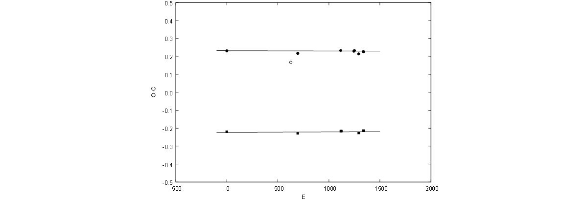
Fig. 1 The O − C variations of V990 Her. Circles and squares represent primary and secondary minima, respectively. The open circle represents the minimum time which is not used in the analysis. Solid and dashed lines are for the theoretical model given in Table 3. 

According to the results given in Table 3, V990 Her has an apsidal motion with a period of U = 14683 ± 2936 years. Due to the relatively long apsidal period compared with the time span of about 30 years which is covered by the observations, the apsidal motion parameters have larger errors. Therefore, the results given in Table 3 should be considered as a preliminary ones. Thus, for V990 Her more observations, which will be performed in the future, are essential.

3.2. Spectroscopic Orbital Parameters

MgII, SiII, FeI, FeII and HI lines can be clearly seen in the spectrum of V990 Her. RVs were obtained from the orders containing the relatively sharp lines of MgII (4481Å), FeI (4957Å), FeI (5616Å) and HI (6563Å). The studied regions are shown in Figure 2. From top to bottom along the y-axis in Figure 2, the normalized spectra are plotted in accordance with the decreasing HJD times given in Table 1.

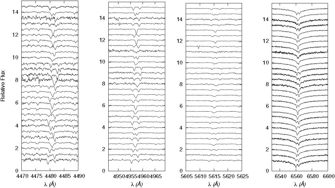
Fig. 2 Analyzed spectral lines. From top to bottom along the y-axis, the normalized spectra are plotted in accordance with the decreasing HJD times given in Table 1 in each panel. 

Gaussian profiles were applied to the central parts of the lines to measure the RVs and then a barrycentric correction was applied to correct the RVs. Measured RVs were listed in Appendices A, B, C and D. The least squares method has been applied to fit the RV equation to the measured RVs. We used the orbital period derived in equation (1) and fixed it during the iterations. The measured RVs and fitted curves (solid red lines) are shown in Figure 3 for each selected line separately. The spectroscopic orbital parameters, such as the longitude of the periastron, ω, orbital eccentricity, e, mass ratio, q = K ₁ /K ₂ and velocity semi-amplitude of the components, K _1,2, were obtained from different lines and their arithmetic mean values are given in Table 4.

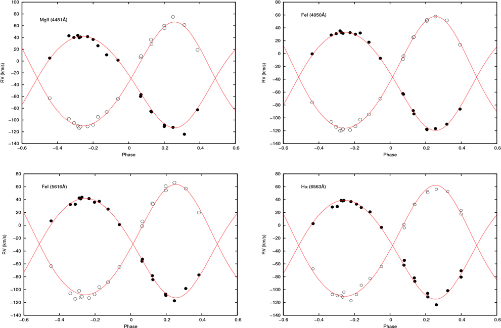
Fig. 3 RVs observations (symbols) and fitted models (red lines) for different spectral lines. Black dots and circles denote the primary and secondary components. The color figure can be viewed online. 

3.3. Photometric Elements

The previously mentioned three photometric data sets obtained in V RI bands were used for the photometric analysis of V990 Her to determine the photometric elements of the system and the light contributions of the components at different phases, which were used to model the component spectra in § 3.4 and § 3.5. The LC solutions were performed with the program phoebe 1.0 (^{Prša & Zwitter 2005}), which is an extension of the wd program (^{Wilson & Devinney 1971}).

The improved light elements given in equation (1) were used in the LCs analysis. The effective temperature of V990 Her was given as T _eff = 7514 K by ^{McDonald et al. (2012)}. However, we obtained a more reliable temperature for the primary component as T _eff1 = 8000 K directly from the spectrum of the system (see § 3.5). The temperature for the primary component T _eff1, the improved period given in § 3.1, the eccentricity e, and the mass ratio q given in Table 4 were fixed during the LC solution. Convergence was allowed for the orbital inclination i, the longitude of the periastron point ω, the dimensionless surface potentials of the components Ω₁ and Ω₂, the effective temperature of the secondary component T _eff,2 , and the relative monochromatic luminosity of the primary component l ₁ /l _tot. The bolometric albedos A _1,2 and gravitational darkening coefficients g _1,2 were adopted as 1.0, as suggested for early-type stars. The bolometric limbdarkening coefficients x _bol1,2 were computed automatically by phoebe 1.0 with the internal tables of the programme which were generated according to the models given by ^{van Hamme (1993)}. The results of the solution are listed in Table 5.

3.4. Disentangling the Components Spectrum

One of the advantages of having numerous spectra taken at different phases is that they allow to obtain the spectrum of the components separately. Thus, we used the korel program provided by ^{Hadrava (1995)} which needs approximate orbital elements and the light contributions of the components at the phases in which the individual spectrum were taken. The orbital parameters and light contributions of the components obtained in § 3.2 and § 3.3 were used as initial values for the korel solution. The orbital period P given in equation (1) was used and fixed during the iterations. The korel solution gives the RVs (see Table 6) of the components and the orbital parameters (see Table 7) of the binary system. The korel solution agrees very well with those obtained from individual lines (see Table 4). The disentangled spectra in the H _α region for both components can be seen in Figure 4.

Fig. 4 Disentangled spectra in H _α region for the primary (left panel) and the secondary (right panel) components of V990 Her obtained from korel solution. The red solid lines represent the synthetic spectra calculated in § 3.5. The color figure can be viewed online. 

3.5. Atmosphere Modelling

We have a spectrum of the system in the middle of the secondary minimum of the LC where ≈45 percent of the light of the secondary component is eclipsed. When the similar physical properties of the components (see Table5) are taken into consideration, it can be regarded as a useful spectrum for a temperature estimation of the primary component.

We know that the components are not early type since there are no He I lines in the composite or disentangled spectra, which means that their temperature is no higher than ≈ 10000 K, and therefore, the local thermodynamic equilibrium assumption could be used to construct the atmosphere models. atlas9 atmosphere models computed by ^{Castelli & Kurucz (2004)} and synthe program of ^{Kurucz (1993)} were used for the generation of the atmospheric models and the synthetic spectra for the components. In the atlas9 code, Z=0.03 and ξ = 2 km s⁻¹ were assumed for the metallicity and micro turbulence velocity, respectively. This method has been applied to the wavelength regions where the dominant lines reside. In Figure 5, the observational data and the synthetic spectra are given for four different wavelength regions as examples.

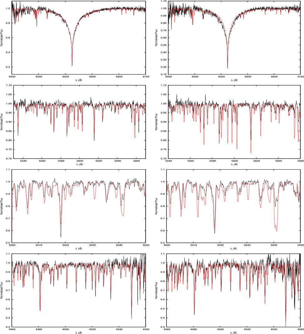
Fig. 5 The observed spectra taken during the secondary (left panel) and primary (right panel) minimum. The synthetic models are shown with red solid lines. The color figure can be viewed online. 

The atmospheric model parameters of the primary component, such as the temperature, T _eff1=8000 ± 200 K, the surface gravity, logg ₁ = 4.0 ± 0.1 and the rotational velocity v _rot1 =28 ± 5 km s⁻¹ were determined.

Moreover, we have a spectrum at orbital phase φ = 0.0. Using a similar approach, the atmospheric model parameters of the secondary component were estimated as T _eff2=7500±200 K, log g ₂=4.0±0.1 and v _rot2 =25±5 km s⁻¹. At three different orbital phases (φ = 0.699, 0.533, 0.290), the synthetic spectra of the components were combined using their light contributions and their specific RVs. The observed spectra taken at the indicated maximum phases and the combined theoretical spectra are shown together in Figure 6.

Fig. 6 The composite synthetic models (red solid lines) fitted to the observed spectra around FeI (5616Å) and HI (6563Å) lines. Each row refers to orbital phases at ϕ = 0.699 (upper panels), 0.533 (middle panels) and 0.290 (bottom panels). The color figure can be viewed online 

3.6. Simultaneous Radial Velocity and Light Curves Solution

The RVs of the components obtained from the korel solution and the multi-colour LCs of the system were analyzed simultaneously with phoebe 1.0. The initial orbital parameters were used from the averaged values given in Tables 4 and 7. We used the improved light elements given in equation (1). The orbital period P and the effective temperature of the primary component T _eff1 were fixed as in § 3.3, the other orbital and photometric parameters were all adjusted in the analyses.

The results of the simultaneous solution are listed in Table 8. The observed LCs in VRI bands and the radial velocity curves (RVCs) of the components are shown along with the theoretical models in Figure 7. The Roche geometry of V990 Her at phases φ=0.0, 0.25 and 0.45 can be seen in Figure 8.

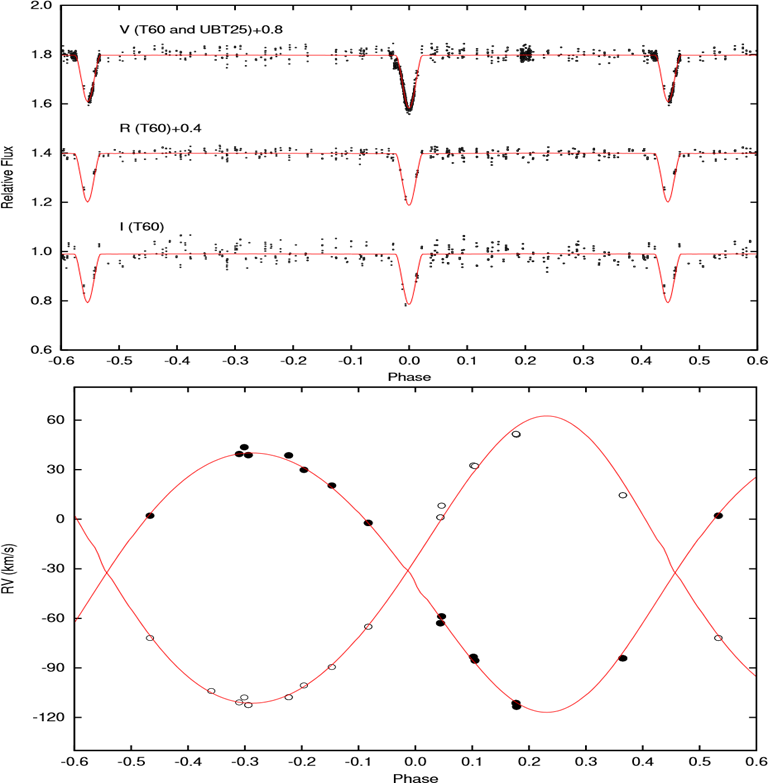
Fig. 7 The theoretical representations of the observed LCs of the system in VRI bands (upper panel) and the observed RVCs of the components (lower panel). The V and R band LCs are shifted 0.8 and 0.4 mag, respectively, for a better illustration. Each row refers to orbital phases at φ = 0.699 (upper panels), 0.533 (middle panels) and 0.290 (bottom panels). The color figure can be viewed online. 

Fig. 8 The Roche geometry of V990 Her at the phases φ = 0.00 (upper panel), φ = 0.25 (middle panel) and φ = 0.45 (lower panel). 

4.1. Physical Properties and Evolutionary Status

Using the parameters given in Tables 7 and 8, the astrophysical parameters of the components and the distance of V990 Her were derived and are given in Table 9. The masses of the components (2.01±0.07 M⊙ and 1.83±0.03 M⊙) correspond to main sequence stars of spectral type between A3-A5 (^{Straizys & Kuriliene 1981}). The evolution status of the components according to the T _eff and log L values given in Table 9 is shown in Figure 9 along with the theoretical evolutionary tracks taken from ^{Bressan et al. (2012)}. The isochrone in Figure 9 was taken from ^{Girardi et al. (2000)}.

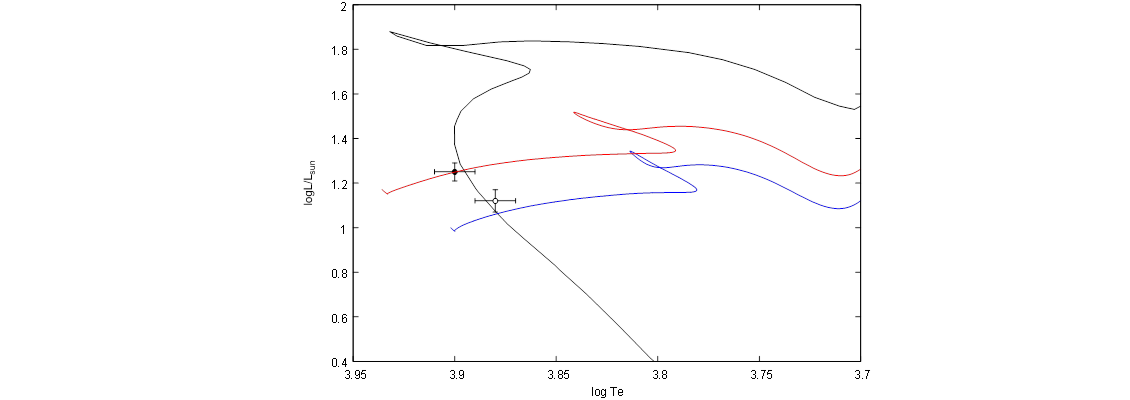
Fig. 9 Comparison of components with evolution models (Black dot and circle represent the primary and secondary components, red and blue solid lines indicates evolution models for Z=0.03 for a 2.00M⊙ and 1.825M⊙ star individually). Black dashed line represents isochrone corresponds 6.3×108yrs for Z=0.03. The color figure can be viewed online. 

Bolometric corrections (BC) for the primary and secondary components were calculated as 0.027 and 0.034 mag using T _eff-BC tables of ^{Flower (1996)}. The bolometric magnitudes M _bol given in Table 9 and BCs were used to derive the absolute magnitudes of the components as M _V1 = 1 ^m .60 ± 0.11 and M _V2 = 1 ^m .93 ± 0.12, respectively. By using the V _J = V _T −0.09×(B _T −V _T ) relation and Tycho magnitudes (B _T = 7 ^m .950, V _T = 7 ^m .710) given by ^{Esa (1997)}, we derived the total visual magnitude of the system as m _V = 7 ^m .688. To obtain the E(B − V ) color excess and the distance of the system we used the total u ⁰ g ⁰ r ⁰ i ⁰ z ⁰ magnitudes of the system given by ^{Pickles & Depagne (2010)} in the following transformation relationships of ^{Smith et al. (2002)}:

Using the light contribution of the components given in Table8 together with the IC magnitudes of the system estimated by equations 3-5 and the (B − V ) − (V − I _C) tables given by ^{Cousins (1981)}, we obtained the (B − V ) colors as 0.185 and 0.250 mag for the primary and secondary components, respectively. For the unreddened (B − V )₀ colors of the components we used the T _eff-(B − V )₀ tables of ^{Flower (1996)} and obtained the values of (B − V )₀ as 0.162 and 0.234 mag, which correspond to E(B − V ) values of 0.023 and 0.017 mag for the primary and secondary components, respectively. Thus, we adopted an average color excess of E(B − V ) = 0.020 mag and as a result we obtained the distance of the system as d = 212 ± 21 pc. Alternatively, an E(B − V ) = 0 ^m .066 value estimated from stilism maps given by ^{Kervella et al. (2019)} corresponds to a distance of d = 198±19 pc. However, our photometric distance value matches better the value of 235 pc given by Gaia which corresponds to a parallax of µ = 4.25 ± 0.08 mas (^{Gaia Collaboration et al. 2016}; ^{Lindegren et al. 2021}) within the given uncertainty box.

4.2. Apsidal Motion and Internal Structure Constant

To test the observed preliminary results concerning the apsidal motion of V990 Her given in § 3.1, we can use the results of previous section. As is known, the total apsidal motion in a binary system occurs mainly for two contributions: (1) a classical part which is due to tidal interactions of the oblate components, and (2) a relativistic contribution which is a direct result of the General Relativity Theory.

The relativistic contribution w˙rel (in degrees per orbital cycle) to total apsidal motion is given by (see ^{Giménez 1985)}:

which was first derived by ^{Levi-Civita (1937)}. Here, m _1,2 are the masses of the components in units of solar mass, e is the orbital eccentricity and P is the orbital period in units of days. By using the related parameters given in Tables 3 and 9 we obtained w˙ _rel = 0^◦ .00033 cycle⁻¹ and so w˙ _cl = 0^◦ .00022 cycle⁻¹.

On the other hand, the relation for the classical part of the apsidal motion rate was given by ^{Kopal (1978)} as follows

where k _2i (i=1, 2) are internal structure constants (ISCs) of the components, while c _2i are as follows

Here Ri/a and wi/wk are the relative radii and and rotational angular velocity for the corresponding component, respectively, wk=2πP is the orbital (Keplerian) angular velocity and P is the orbital period of the system. The f and g functions of the orbital eccentricity e are given by

Using the apsidal and absolute parameters given in Tables 1 and4 we obtained the observed average ISC for the system as k¯2 = 0.0035±0.0008.

To obtain the theoretical ISCs of the components we used the stellar models given by ^{Claret & Gimenez (1992)}, which assume X=0.649, Z=0.03 and take mass loss and core overshooting into account. By the interpolation we obtained log L=1.30 and 1.13L⊙, Teff=8222 and 7621K, Age=5.72×108 and 7.89×108 years and k2=0.0032 and 0.0031 for the primary and secondary components, respectively. These results correspond to a value of k¯2theo=0.0032 and w˙cltheo=0∘.00019cycle​-1. Consequently, the theoretical value of the total apsidal motion rate is obtained as w˙theo=0∘.00052cycle​-1. On the other hand, by taking the weighted average of the ages of the components with the corresponding ci we obtained the age of the system as 6.74×108years.