


Servicios Personalizados
Revista
Articulo
 texto en
  Inglés (pdf)
 Artículo en XML
 Referencias del artículo
 Enviar artículo por email
Indicadores
-
 Citado por SciELO
 -
 Accesos
Links relacionados
-
 Similares en
SciELO
Similares en
SciELO
Compartir

 Permalink
Tecnología y ciencias del agua
versión On-line ISSN 2007-2422
Tecnol. cienc. agua vol.11 no.3 Jiutepec may./jun. 2020 Epub 10-Jun-2024
https://doi.org/10.24850/j-tyca-2020-03-04
Articles
Detection of homogeneous records in 16 large series of annual precipitation of the Potosino Plateau, Mexico
1Profesor jubilado de la Universidad Autónoma de San Luis Potosí, San Luis Potosí, México, campos_aranda@hotmail.com
Homogenization methods have been developed to reduce the impact of non-climatic alterations in the records or series of data coming from climatological stations. Such impacts arise from changes either in the location of the station, in the equipment used or in the measurement technique, as well as from alterations suffered by the surroundings. Due to the fact that the historic information on the changes that occurred in the climatological station is generally not available, statistical tests are used to detect breaking points that imply changes in the mean and, therefore, loss of homogeneity of the record. There are two approaches to the application of statistical tests: (1) individually to each record to be tested and (2) using reference series based on neighboring stations. In this study, the first approach was applied to a specific geographical area and using the following four tests: Von Neumann, Pettitt, Buishand and SNHT. Sixteen annual precipitation series of the Potosino Plateau of Mexico were processed in the common period from 1964 to 2016, the amount of values varied from 42 to 53 data. Monthly data were used; hence, the procedures to deduce missing values and to detect and correct extreme maximums are exposed. A description of how the missing annual values were estimated is also included. It was found that 11 records were reliable, because no test detected them as non-homogeneous. Three records were classified as less reliable, because a maximum of two tests found them non-homogeneous and finally, two records are unreliable, since a minimum of three tests find them non-homogeneous. The adopted procedure proposes a practical strategy to detect homogeneous records of annual precipitation; its advantages are exposed at the study.
Keywords: homogenization; maximum outliers values; von Neumann test; Pettitt rank test; Buishand rank test; SNHT test; monthly and annual rainfall
Los métodos de homogenización han sido desarrollados para reducir el impacto de las alteraciones no climáticas en los registros o series de datos procedentes de las estaciones climatológicas. Tales impactos proceden de cambios en la ubicación de la estación, en el equipo utilizado y en la técnica de medición, así como por las alteraciones que sufre su entorno. Debido a que la información histórica sobre los cambios ocurridos en la estación climatológica por lo general no está disponible, se recurre a aplicar pruebas estadísticas para detectar puntos de quiebre que implican cambios en la media y, por lo tanto, pérdida de homogeneidad del registro. Existen dos enfoques de aplicación de las pruebas estadísticas: (1) de manera individual a cada registro por probar y (2) haciendo uso de series de referencia, formadas con base en estaciones circunvecinas al registro que se prueba. En este estudio se aplicó el primer enfoque, en una zona geográfica y haciendo uso de las cuatro pruebas siguientes: Von Neumann, Pettitt, Buishand y SNHT. Se procesaron 16 series de precipitación anual del Altiplano Potosino de México, en el periodo común de 1964 a 2016, cuya amplitud varió de 42 a 53 datos. Se trabajó con datos mensuales, y por ello se expone cómo se dedujeron los valores faltantes, y cómo se detectaron y corrigieron los máximos extremos. También se describe cómo se estimaron los valores anuales faltantes. Se encontró que 11 registros resultaron confiables debido a que ninguna prueba los detectó como no homogéneos. Tres registros se clasificaron como menos confiables, pues un máximo de dos pruebas los encontró no homogéneos y, por último, dos registros son no confiables, ya que un mínimo de tres pruebas los encuentra no homogéneos. El procedimiento adoptado formuló una estrategia práctica para detectar registros homogéneos de precipitación anual, cuyas ventajas se exponen en el estudio.
Palabras clave: homogenización; valores máximos dispersos; test de Von Neumann; test del rango de Pettitt; test del rango de Buishand; prueba SNHT; precipitación mensual y anual
Introduction
Overview
Seemingly, extreme weather events are becoming more severe and frequent, with their respective devastating impacts; in addition, perhaps they are caused by climate change. These two statements require that statistical analyses oriented to their prediction and forecast be based on quality meteorological and climatic data, that is, that they be accurate and homogeneous. In fact, obtaining perfectly homogeneous records or large series of climatic data is almost impossible, due to the inevitable change of the area surrounding the site of the climatological station, which affects the observed data. The loss of homogeneity occurs when there are changes in the record generated by non-climatic causes (Guijarro, 2014; Yozgatligil & Yazici, 2016).
In summary, all records or data series that are measured at climatological stations often undergo alterations that are not related to climate variations. Such modifications arise from changes in the location of the station, by replacing its instruments or changing the measurement technique and by altering the physical conditions surrounding the site. Homogenization is a procedure to detect and correct the aforementioned artificial alterations. Regarding homogenization techniques, Guijarro (2014) briefly describes them and focuses on the available computing packages. A series of climatological data is considered homogeneous, when the measurement conditions at the station have not changed over time (Beaulieu et al., 2008). Guijarro (2014) highlights the importance of the Meteorological Services in avoiding by all means, changes that affect the climatological measurements, since this makes the use of homogenization methods unnecessary.
The volcanic eruptions, being a natural phenomenon that causes an alteration of climate records, define change points that do not imply loss of homogeneity. On the contrary, break points are change points caused by non-climatic alterations and therefore imply loss of homogeneity (Toreti et al., 2011).
The homogenization of the climatic series is a difficult task that must be carried out with extreme care, especially when additional data or historical data (metadata) of the climatological station are not available; common case. The objective of homogenization is to eliminate, or at least reduce, non-climatic alterations, while the climatic signal is preserved (Toreti et al., 2011). Many methods have been proposed to homogenize the climatological series, a complete review that includes suggestions for their use can be found in Peterson et al. (1998), and in Beaulieu, Ouarda and Seidou (2007).
A first classification of the procedures and/or statistical tests that detect and correct the loss of homogeneity, establishes two groups: the first is based on the availability of additional data on the historical evolution of the climatological station, known as metadata and the second in the absence of such data. Rhoades and Salinger (1993) present techniques for the first group, under two approaches: (1) using neighboring stations and (2) in stations isolated or from old or primigenial records. In general, the historical data of the climatological station are essential to validate the changes detected by the tests and unfortunately, they are almost always not available.
Another classification of homogenization techniques divides them into: absolute tests, which exclusively use the series or record under analysis and relative tests, which use close or correlated records to form the reference series. Both approaches are valid and useful, and both also exhibit disadvantages. Yozgatligil and Yazici (2016) compare seven tests of each type and find that the relative tests have better performance, among them they cite first the standard normal homogeneity test, designated SNHT.
Syrakova and Stefanova (2009) indicate that due to the difficulty in establishing a priori which stations are homogeneous, they choose to follow an iterative scheme of gradual homogeneity improvement, which was proposed by Hanssen-Bauer and Forland (1994), and has been also applied by Moberg and Alexandersson (1997); González-Rouco, Jiménez, Quesada, and Valero (2001), and Tuomenvirta (2001).
Instead, Wijngaard, Klein Tank and Können (2003) apply and cite two advantages of the absolute tests: (1) easy application in sparse networks and (2) superior to relative tests in networks with simultaneous changes, since these do not detect them. Dhorde and Zarenistanak (2013) use a mixed approach in the study of homogeneity of 20 climatological stations, applying the Pettitt and SNHT tests to each series and the SNHT test for gradual changes in the mean with reference series.
Ducré-Robitaille, Vincent and Boulet (2003) evaluated 8 homogenization techniques of temperature series, using homogeneous simulated series and containing one or several changes in the mean (steps). They found that most have a good performance, but two of them tend to be more efficient: the SNHT test and the multiple linear regression technique.
Beaulieu et al. (2008) also compared eight statistical tests to detect lack of homogeneity in annual precipitation series, using several thousand synthetic series both homogeneous and non-homogeneous and found that no method is efficient in all types of loss of homogeneity, but three of them have a much better perform: the bivariate test, the Jaruskova method and the SNHT test.
In Mexico, and specifically for the state of Veracruz, Guajardo-Panes, Granados-Ramírez, Sánchez-Cohen, Díaz-Padilla and Barbosa-Moreno (2017), have applied the absolute approach with the SNHT, Pettitt and Buishand tests, under a spatial verification scheme, to select neighboring climatological stations to the station being tested, within the same climatic unit, defined this based on the variation interval of the climate element being analyzed. The above is equivalent to processing climate information by sub-regions or climatic zones.
Quality control concept
González-Rouco et al. (2001) have defined that the quality control processes of the climatic data series involve three stages: (1) detection and correction of outliers; (2) interpolation techniques of missing data and (3) homogenization of the series. In fact, the estimation of missing data occurs at monthly level, before and after homogenization, when trying to complete series to have a common information period. Due to the fact that all climatic data series are extremely sensitive to the presence of erroneous values and scattered data, Eischeid, Baker, Karl and Diaz (1995) address the detection and correction of scattered (outlier) data according to an objective approach of temporary verification in the analyzed and spatial record based on six interpolation techniques of monthly data.
Objective
A practical approach or strategy for verifying homogeneity in annual precipitation records has been formulated, which has the following relevant characteristics: (1) work by geographic regions or sub-regions, using monthly data; (2) missing monthly data are estimated using a statistical technique; (3) details how extreme maximum monthly values are verified and corrected, by truncation; (4) missing annual data are deduced, with a regional weighting technique; (5) an absolute contrast approach is used, using four statistical tests (Von Neumann, Pettitt, Buishand and SNHT) and (6) each record that was not homogeneous or reliable is checked graphically and the loss of homogeneity is corrected when there is a breaking point. In this study we worked on the semi-arid climatic region of the Potosino Plateau of Mexico, processing 16 long-term records, whose number of annual data varied from 42 to 53.
Operative methods
Correction of outliers
Outliers are values that are far from the trend shown in a set of data, which correspond to erroneous measurements or extreme meteorological events. There are several approaches to contrast and verify the temporal and/or spatial variability of the climatic variable studied, in order to identify the outliers and diagnose when they are erroneous data or feasible values to occur. When the outliers are undoubtedly wrong observations, such data is deleted and then there is a problem of missing data. When they are feasible values, it must be decided whether they are corrected and how it should be done (Eischeid et al., 1995; González-Rouco et al., 2001).
Due to the practical difficulties involved in the verification of outliers in the original or field records, an approach to reducing the scattering in the right tail of the probability distribution was adopted, to seek a better performance of homogenization techniques that are not resistant (Lanzante, 1996). Such approach is to limit the outliers to an extreme threshold magnitude (P vd ), which is (Eischeid et al., 1995):
where, P 50 is the median or the percentile of the 50%, P 75 and P 25 are the percentiles of the 75% and 25% and FM is the interquartile range multiplication factor (RIC), with an empirical value adopted of 2.75 for average temperature data and 4.00 for precipitation, both monthly. González-Rouco et al. (2001) use a similar expression for their monthly precipitation data:
The outliers superior to P vd are replaced by such limit. This truncation approach of the outliers reduces the bias that they originate and also maintains information relative to the extreme values. Eischeid et al. (1995)) indicate that RIC is used in quality control processes because it is resistant (Lanzante, 1996) to outliers. In this study the criterion defined by equation 1 was adopted, having a greater theoretical and empirical justification.
Absolute Approach Tests
The tests that are applied to the series studied are those of the Wijngaard et al. (2003) who uses four methods to test the loss of homogeneity, these are: the Von Neumann test, the Pettitt range test, the Buishand range test and the SNHT test. These four tests assume that under the null hypothesis the annual values of the series (Y i ) of the variable Y that are studied, are independent and are identically distributed. Under the alternative hypothesis, the first test assumes that the series is not randomly distributed and the remaining three consider that there is a change in the mean or break point. Under the alternative hypothesis -the first test-, it is assumed that the series is not randomly distributed and the remaining three consider that there is a change in the mean or break point. Logically, the homogeneity or consistency of the series implies that their data belong to a single population that has an invariant mean over time (Machiwal & Jha, 2012).
The Pettitt, Buishand and SNHT tests can locate the year where the break point probably occurs and, in general, they are different in their approach or conception. It has been found that the first two are more sensitive to the break points that occur around the middle of the series; on the contrary, the SNHT test detects changes more easily at the start and end of series.
Von Neumann, Buishand and SNHT tests assume that the Y i data have normal distribution; on the other hand, Pettitt's test does not require such consideration, since it is based on the ranges and not on the values of the series, which also makes it less sensitive to outliers. The Von Neumann test is considered complementary to the other three, because it detects loss of homogeneity due to causes other than the change in the mean (Wijngaard et al., 2003).
Von Neumann test
The Von Neumann quotient (N) has in the numerator the sum of the successive squared differences and in the denominator the variance. Its equation is (Wijngaard et al., 2003):
in which, n is the number of years of the series or processed record. When the series is homogeneous N has a value close to two, if there is a change in the mean, N decreases and is less than the critical value (Table 1); when there are rapid variations in the mean, N increases and can be higher than two. Wijngaard et al. (2003) show their critical values in Table 1, obtained by other authors, which are a function of n and of the level of significance (α) of the test.
Table 1 Critical values of the four absolutes tests applied, with significance level (α) of 5% and 1% (Pettitt, 1979; Wijngaard et al., 2003; Khaliq & Ouarda, 2007).
| Data No. (n) | Von Neumann test | Pettitt range test | Buishand range test | SNHT test | ||||
|---|---|---|---|---|---|---|---|---|
| 5% | 1% | 5% | 1% | 5% | 1% | 5% | 1% | |
| 20 | 1.30 | 1.04 | 64.8 | 80.3 | 1.43 | 1.60 | 6.95 (7.089) | 9.56 (9.113) |
| 30 | 1.42 | 1.20 | 118.0 | 146.3 | 1.50 | 1.70 | 7.65 (7.747) | 10.45 (10.153) |
| 40 | 1.49 | 1.29 | 181.0 | 224.4 | 1.53 | 1.74 | 8.10 (8.151) | 11.01 (10.771) |
| 50 | 1.54 | 1.36 | 252.3 | 312.8 | 1.55 | 1.78 | 8.45 (8.432) | 11.38 (11.193) |
| 70 | 1.61 | 1.45 | 416.8 | 516.7 | 1.59 | 1.81 | 8.80 (8.814) | 11.89 (11.737) |
| 100 | 1.67 | 1.54 | 710.1 | 880.5 | 1.62 | 1.86 | 9.15 (9.167) | 12.32 (12.228) |
Pettitt range test
The ranges (R 1, R 2,..., R n ) of the original series (Y 1, Y 2,...., Y n ) are used to calculate the test statistics (Pettitt, 1979; Wijngaard et al., 2003; Yozgatligil & Yazici, 2016):
The calculation of the ranges is quite simple, first the data are ordered in increasing form and then each data ordered is compared against all the originals, when they coincide that is the range sought. If a break point occurs in year k, then the statistical (P k ) is maximum or minimum near such year and its absolute maximum value exceeds the critical value of Table 1, which is defined by the following equation as a function of level of significance (α) and n (Pettitt, 1979; Dhorde & Zarenistanak, 2013):
The graph of k in the abscissa against P k in the ordinates shows the test results. Mallakpour and Villarini (2016) analyze with simulation the performance or sensitivity of the Pettitt test in the detection of sudden changes in the mean, in very different conditions and in series of extreme values.
Buishand range test
We begin by calculating the residual mass curve, defined as (Buishand, 1982; Wijngaard et al., 2003):
When the series is homogeneous, the values of
The critical values of R/(
SNHT test
The statistic T k of the test compares the standardized mean of the first k years of the record against that relative to the following (n - k) years (Alexandersson, 1986; Wijngaard et al., 2003; Syrakova & Stefanova, 2009):
with:
This statistics has a behavior equal to P k , with its critical values defined in Table 1. In parentheses, the critical values recently developed by Khaliq and Ouarda (2007) have been cited which are more accurate than the original ones, covering large samples and have been exposed to six levels of reliability (1-α), varying from 90% to 99%. Alexandersson and Moberg (1997) present the version of the SNHT test for series or linear trend records.
Toreti et al. (2011) cite the results of several authors and verify based on 1000 synthetic series of 100 years of non-homogeneous length, that the SNHT test is prone to detect breakpoints at the beginning or end of the series, when it has few data and therefore avoid applying it in segments with less than ten values.
Regarding the level of significance (α) to be used in the SNHT test, Syrakova and Stefanova (2009) accept the criteria of Hanssen-Bauer and Forland (1994), and González-Rouco et al. (2001) to use 10% if the break point is verified by the historical data of the climatological station and 5% if there is no such verification. This selection reduces the risk of accepting homogeneity in the absence of data on changes occurred in the climatological station, location, equipment and measurement technique.
Correction of loss of homogeneity
When a break point has been identified in an annual precipitation record, the data prior to such change are corrected, by multiplying them by the following factor (González-Rouco et al., 2001):
being,
Classification of the series tested
The classification depends on the number of tests that rejected the null hypothesis, defining three categories whose designations according to Wijngaard et al. (2003), and Dhorde and Zarenistanak (2013) are: useful, doubtful and suspect and according to Guajardo-Panes et al. (2017) are reliable, moderately reliable and unreliable. In this study the following designation is adopted: in class 1 or “reliable” the series that were homogeneously detected by the four tests are grouped; or, only one test detected loss of homogeneity; class 2 or “less reliable” includes series with two tests that detect a lack of homogeneity and class 3 or “unreliable” are series with three or four tests that reject the null hypothesis.
With the class 1 series, trend analysis and climate variability studies can be performed; with class 2, the results of the aforementioned analyses should be kept in reserve, but they are feasible if there are no other reliable series available and the class 3 series should not be used for the aforementioned estimates.
There is a notable difference in establishing the previous classification, since Wijngaard et al. (2003) define a level of significance (α) in the tests of 1% and instead, in the other two works mentioned 5% is used. In this study, α = 5% was accepted, to coincide with the recommendations of the SNHT test (Alexandersson, 1986).
Data used and auxiliary techniques
Selection of climatological stations
This study used the monthly climatological information from the Excel file provided by the San Luis Potosí Local Agency of the National Water Commission (CONAGUA), which is grouped into the three geographical areas of the state: Potosino Plateau, Middle Zone and Huasteca Region. Processed data records correspond to the climatic variable annual precipitation in millimeters, each data integrated by the sum of the twelve monthly rainfall values.
The Potosino Plateau archive covers more than 60 climatological stations, but some are repeated because they belong to the extinct Ministry of Water Resources and the National Meteorological Service. From such availability, stations with less than 40 years of registration and lapses of missing years were eliminated. With such restrictions a sample of 16 stations was obtained whose initial year of their records is indicated with AI in Table 2 and Table 3 of data to be processed. All records cover until 2016, with the exception of the Los Pilares station that was suspended in 2009.
Table 2 Values of the annual precipitation (millimeters) and its statistics in the eight indicated pluviometric stations of the Potosino Plateau, Mexico.
| No. | 1 | 2 | 3 | 4 | 5 | 6 | 7 | 8 |
|---|---|---|---|---|---|---|---|---|
| Year | Vanegas | S. M. del Refugio | La Presa | Matehuala | La Maroma | Charcas | Palo Blanco | Reforma |
| 1964 | 282.0 | 302.6 | - | (614.5) | - | (283.1) | 211.0 | - |
| 1965 | 300.8 | 319.0 | - | 464.0 | 312.5 | 317.0 | 350.5 | 374.5 |
| 1966 | 457.6 | 377.0 | - | 766.0 | 408.0 | 463.7 | 586.0 | 598.7 |
| 1967 | 410.9 | 362.3 | - | 578.0 | 462.9 | 585.5 | 910.0 | 580.3 |
| 1968 | 440.4 | 330.5 | - | 662.0 | 490.0 | 598.0 | 472.0 | 393.3 |
| 1969 | 713.7 | (127.9) | - | (420.5) | 248.0 | 163.0 | (242.2) | 247.9 |
| 1970 | 325.0 | 282.0 | - | 368.5 | 205.0 | 517.0 | 196.0 | 300.0 |
| 1971 | 224.5 | 390.5 | - | [327.5] | 387.0 | 684.0 | 509.7 | 268.3 |
| 1972 | 253.9 | 329.0 | - | 533.5 | 280.0 | (389.7) | 461.1 | (255.9) |
| 1973 | 404.0 | 513.6 | - | 471.0 | 434.4 | 607.6 | 168.6 | *1037.3* |
| 1974 | 82.4 | 107.0 | - | (328.9) | 95.0 | (175.0) | 191.8 | 248.6 |
| 1975 | 155.5 | 163.5 | (247.1) | 526.0 | 332.0 | [364.3] | 329.5 | 277.0 |
| 1976 | 336.0 | 501.3 | 695.3 | 891.8 | 586.0 | 949.5 | 491.6 | 650.3 |
| 1977 | 152.5 | 136.1 | 470.2 | 532.6 | 355.0 | 199.7 | 261.3 | 224.0 |
| 1978 | 249.4 | 252.7 | 570.5 | 698.3 | 439.0 | 376.6 | 335.3 | 344.1 |
| 1979 | 222.3 | 223.1 | 383.2 | 441.9 | 303.0 | 263.9 | 238.6 | 225.9 |
| 1980 | 346.0 | (249.5) | 428.9 | 474.6 | 311.0 | 330.4 | (172.4) | 293.1 |
| 1981 | 249.9 | (178.8) | 590.2 | [438.5] | 346.0 | 364.5 | (211.0) | 424.3 |
| 1982 | 288.5 | 265.1 | 394.0 | (274.3) | 360.0 | 166.6 | (297.4) | 320.7 |
| 1983 | 457.1 | 358.6 | 444.9 | 568.0 | 268.0 | 192.8 | 194.0 | 230.3 |
| 1984 | 276.8 | 370.7 | 649.2 | 369.0 | 440.0 | 599.5 | 227.5 | 342.2 |
| 1985 | 251.4 | 233.1 | 636.9 | [475.4] | 392.0 | 507.5 | 122.6 | 370.4 |
| 1986 | 221.8 | 240.0 | 377.4 | *668.3* | 288.0 | (326.7) | 184.3 | 258.4 |
| 1987 | 417.8 | (77.0) | 591.2 | 593.9 | 499.0 | 591.1 | 148.2 | 319.9 |
| 1988 | 329.6 | 38.7 | 634.5 | 557.2 | 359.8 | (443.6) | (155.5) | 465.2 |
| 1989 | 122.1 | 139.0 | 401.3 | (491.7) | 212.0 | 344.0 | (31.0) | 136.8 |
| 1990 | 341.0 | 355.9 | 466.5 | (648.2) | 327.0 | (505.7) | 135.0 | 432.9 |
| 1991 | 336.4 | 305.0 | 508.6 | 695.2 | 497.1 | 659.3 | [554.5] | 497.8 |
| 1992 | 351.6 | 383.0 | 597.1 | 677.3 | 391.0 | 773.0 | 255.0 | 540.5 |
| 1993 | 185.5 | *884.9* | 411.0 | 445.2 | 256.0 | 612.3 | 121.0 | 283.1 |
| 1994 | 95.0 | 371.5 | 464.9 | 571.1 | 426.0 | 227.7 | 171.0 | 480.4 |
| 1995 | 52.5 | 241.0 | (461.9) | 559.1 | 351.0 | 119.0 | (264.8) | 419.9 |
| 1996 | 144.5 | 294.1 | 487.1 | 310.3 | 206.1 | 405.7 | 222.3 | 125.1 |
| 1997 | 241.7 | 561.2 | 574.7 | 586.2 | 367.0 | 506.2 | 305.4 | 269.8 |
| 1998 | 190.8 | 112.5 | 316.2 | 334.8 | 244.0 | 393.5 | 250.6 | 325.1 |
| 1999 | 182.5 | 133.0 | 366.4 | 347.6 | 177.0 | 229.1 | (81.8) | 111.5 |
| 2000 | 173.5 | 250.0 | (303.8) | 313.2 | 331.0 | 310.6 | 175.5 | (91.7) |
| 2001 | 176.5 | 184.0 | (377.2) | 431.7 | 367.0 | 545.7 | 200.2 | 232.2 |
| 2002 | 428.0 | 410.0 | (818.0) | 753.1 | 508.0 | 834.8 | 428.8 | 414.3 |
| 2003 | 307.2 | 244.0 | (497.3) | 677.6 | 502.9 | 486.0 | 163.8 | 374.7 |
| 2004 | 225.0 | 404.0 | (701.6) | 648.7 | 387.8 | 742.0 | 245.1 | 356.1 |
| 2005 | 224.0 | 179.0 | 327.1 | 372.0 | 276.0 | 353.8 | 194.1 | 214.6 |
| 2006 | 339.0 | (149.9) | 494.6 | 624.8 | 500.0 | 607.7 | 315.0 | 302.4 |
| 2007 | 351.5 | 72.0 | 854.2 | 549.3 | 474.0 | 758.2 | 462.5 | 513.7 |
| 2008 | 337.0 | 354.5 | 664.5 | 625.5 | 309.0 | 552.6 | 372.0 | 359.3 |
| 2009 | 352.5 | 337.6 | 566.2 | 406.9 | 342.0 | 610.7 | 373.0 | 395.2 |
| 2010 | 327.8 | 371.0 | 496.6 | 503.6 | 593.0 | 607.2 | 330.0 | (155.8) |
| 2011 | 137.0 | 98.0 | 340.5 | 292.3 | 147.0 | 330.0 | 182.0 | 180.6 |
| 2012 | 143.1 | 150.7 | 564.0 | 425.7 | 386.6 | 243.2 | 258.0 | 323.4 |
| 2013 | 536.8 | 563.0 | 973.1 | 726.4 | 687.0 | 889.7 | 398.5 | 601.0 |
| 2014 | 258.8 | 398.5 | 474.9 | 525.1 | 333.0 | 394.0 | 326.0 | 422.1 |
| 2015 | 525.5 | 581.0 | 724.1 | 702.7 | 576.0 | 732.3 | 713.9 | 614.4 |
| 2016 | 281.0 | 486.0 | 630.0 | 668.5 | 351.0 | 356.2 | 207.0 | 427.9 |
| AI | 1964 | 1964 | 1975 | 1957 | 1965 | 1962 | 1964 | 1965 |
| n | 53 | 53 | 42 | 53 | 52 | 53 | 53 | 52 |
| Min | 52.5 | 38.7 | 247.1 | 274.3 | 95.0 | 119.0 | 31.0 | 91.7 |
| Max | 713.7 | 884.0 | 973.1 | 891.8 | 687.0 | 949.5 | 910.0 | 1037.3 |
|
|
287.1 | 297.1 | 523.3 | 527.5 | 367.8 | 464.0 | 290.7 | 358.7 |
| Med | 281.0 | 294.1 | 495.6 | 532.6 | 357.4 | 443.6 | 245.1 | 333.6 |
| Cv | 0.439 | 0.531 | 0.299 | 0.271 | 0.324 | 0.434 | 0.558 | 0.461 |
| Cs | 0.757 | 1.039 | 0.721 | 0.140 | 0.255 | 0.371 | 1.565 | 1.433 |
| Ck | 4.459 | 5.471 | 3.728 | 2.548 | 3.380 | 2.623 | 6.445 | 7.352 |
| r 1 | 0.241 | 0.189 | -0.025 | 0.163 | -0.08 | 0.032 | 0.347 | 0.044 |
Table 3 Values of the annual precipitation (millimeters) and its statistics in the eight indicated pluviometric stations of the Potosino Plateau, Mexico.
| No. | 9 | 10 | 11 | 12 | 13 | 14 | 15 | 16 |
|---|---|---|---|---|---|---|---|---|
| Year | Moctezuma | El Mezquite | El Grito | Los Pilares | Mezquitic | Los Filtros | El Peaje | Villa de Arriaga |
| 1964 | {232.5} | 197.0 | - | 281.6 | 294.5 | 418.0 | 456.1 | 489.0 |
| 1965 | {459.0} | 287.5 | - | 422.0 | 233.0 | 383.6 | 454.2 | 426.1 |
| 1966 | {371.9} | 428.0 | - | 413.0 | 426.5 | 565.2 | 539.0 | 631.7 |
| 1967 | {224.0} | 495.8 | - | 672.8 | 572.1 | 627.3 | 557.6 | 538.0 |
| 1968 | {417.5} | 358.0 | - | 415.3 | 540.9 | 504.1 | 476.0 | (199.9) |
| 1969 | {78.0} | 183.0 | 178.6 | 203.5 | 295.0 | 302.7 | 394.0 | 174.0 |
| 1970 | {333.7} | 250.0 | 380.8 | 323.6 | 348.5 | 363.5 | 369.2 | 269.7 |
| 1971 | 183.0 | 297.0 | 540.3 | 399.5 | 471.0 | 388.6 | 541.0 | 593.0 |
| 1972 | 441.6 | 286.5 | 394.1 | 300.5 | 293.5 | 350.7 | (243.8) | 347.0 |
| 1973 | 307.0 | 760.5 | 530.3 | 379.0 | 545.0 | 420.1 | 388.7 | 328.5 |
| 1974 | 236.6 | 576.9 | 268.9 | 251.0 | 310.6 | 235.9 | (267.1) | 156.9 |
| 1975 | 427.8 | 700.5 | 461.4 | 372.8 | 557.0 | 374.4 | 494.3 | 280.5 |
| 1976 | 463.9 | 523.0 | 607.2 | 508.6 | 756.0 | 503.2 | 631.1 | 359.5 |
| 1977 | 343.3 | 265.8 | 434.3 | 319.9 | 402.2 | 282.8 | 307.2 | 96.0 |
| 1978 | 345.2 | 419.2 | 311.9 | 352.6 | 429.0 | 347.2 | 383.3 | 507.5 |
| 1979 | 325.5 | 361.5 | 270.4 | 393.5 | 380.9 | 354.6 | 355.7 | 192.0 |
| 1980 | 260.7 | 290.0 | 280.4 | 216.5 | 319.9 | 253.9 | 305.8 | 375.5 |
| 1981 | 374.7 | 493.8 | 457.2 | 474.6 | 492.9 | 500.7 | 504.3 | 270.9 |
| 1982 | 334.8 | 321.0 | 467.8 | 298.2 | 305.7 | 326.7 | 291.4 | 292.5 |
| 1983 | 314.3 | 351.4 | 507.2 | 376.8 | 285.1 | 280.4 | 259.3 | 154.5 |
| 1984 | 563.0 | 468.7 | 625.0 | 377.2 | 564.9 | 361.6 | 507.7 | 148.0 |
| 1985 | 594.2 | (355.7) | 534.4 | 437.6 | 478.4 | 489.1 | 485.3 | 167.0 |
| 1986 | 296.1 | [373.4] | 419.2 | 421.0 | 439.7 | 456.7 | 403.2 | 504.0 |
| 1987 | (339.4) | [431.6] | 566.6 | 393.5 | 427.0 | 364.8 | 322.6 | 504.9 |
| 1988 | 531.4 | (337.8) | 672.1 | 536.6 | 576.3 | 455.0 | 399.4 | 256.0 |
| 1989 | (219.1) | 256.0 | 262.8 | 736.2 | 270.5 | 239.5 | 282.9 | 359.5 |
| 1990 | 315.2 | (62.6) | 457.0 | 285.9 | 420.4 | 395.5 | 372.7 | 728.3 |
| 1991 | 491.9 | 33.9 | 539.4 | 492.5 | 641.2 | 528.1 | 476.0 | *876.6* |
| 1992 | 521.9 | 90.0 | 524.9 | 525.2 | 480.8 | 469.6 | 477.1 | 837.0 |
| 1993 | 310.6 | 44.5 | 407.8 | 382.9 | (85.7) | 296.1 | 404.7 | 523.0 |
| 1994 | 430.5 | 358.0 | 563.0 | 472.9 | (178.1) | 332.8 | 348.0 | (562.9) |
| 1995 | 383.6 | (127.8) | 343.1 | 337.3 | 395.4 | 285.7 | 324.7 | 400.0 |
| 1996 | 305.6 | 209.6 | 361.4 | 281.9 | 304.5 | 280.4 | 331.3 | *542.6* |
| 1997 | 407.5 | 361.2 | 551.5 | 458.1 | 270.5 | 432.6 | 439.0 | 679.0 |
| 1998 | 177.8 | 236.0 | 187.0 | 238.9 | 130.7 | 363.7 | 339.3 | 418.0 |
| 1999 | 327.5 | 208.0 | 369.6 | 349.9 | 163.0 | 399.8 | 334.7 | 249.0 |
| 2000 | 222.5 | 292.0 | 1226.4 | 219.8 | 300.0 | 169.6 | 281.9 | 122.0 |
| 2001 | 406.6 | 406.0 | 305.6 | 420.9 | 499.9 | 273.9 | 321.8 | (111.7) |
| 2002 | 495.5 | 693.0 | 593.7 | 525.2 | 642.2 | 466.8 | 556.7 | (112.1) |
| 2003 | 418.7 | 527.0 | 360.5 | 367.1 | 224.7 | 425.7 | 319.0 | 337.0 |
| 2004 | 510.0 | 825.0 | 546.4 | 607.2 | 474.8 | 550.8 | 702.7 | 688.5 |
| 2005 | (224.9) | 232.0 | (210.5) | 350.9 | (357.4) | 295.1 | 273.8 | 287.0 |
| 2006 | 258.0 | 450.0 | 347.0 | 342.4 | 383.0 | 509.8 | 556.4 | 340.0 |
| 2007 | *832.3* | 678.0 | 611.7 | 578.3 | 457.0 | 516.9 | 520.2 | 270.0 |
| 2008 | 353.0 | 434.0 | 268.2 | 437.5 | 590.5 | 373.5 | *562.7* | 546.4 |
| 2009 | 39.0 | 447.0 | 360.5 | - | 448.4 | 464.5 | 533.6 | 201.0 |
| 2010 | 34.0 | 597.2 | 542.0 | - | 508.4 | 492.7 | 563.9 | (263.8) |
| 2011 | 15.0 | 232.0 | 257.1 | - | 327.8 | 218.0 | 291.8 | (75.7) |
| 2012 | 18.0 | 471.0 | 325.5 | - | 286.4 | 195.5 | 244.7 | 134.9 |
| 2013 | 89.0 | 810.0 | 649.0 | - | 822.4 | 548.1 | 626.8 | 189.2 |
| 2014 | 386.0 | 675.0 | 451.0 | - | 448.5 | 387.3 | (364.0) | 165.0 |
| 2015 | 451.0 | 1040.0 | 678.5 | - | 729.7 | 710.2 | 680.3 | (396.5) |
| 2016 | 162.0 | 1040.0 | 389.0 | - | 481.1 | 441.7 | 346.0 | 340.1 |
| AI | 1971 | 1962 | 1969 | 1963 | 1943 | 1950 | 1963 | 1962 |
| n | 53 | 53 | 48 | 45 | 53 | 53 | 53 | 53 |
| Min | 15.0 | 33.9 | 178.6 | 203.5 | 85.7 | 169.6 | 243.8 | 75.7 |
| Max | 832.3 | 1040.0 | 678.5 | 736.2 | 822.4 | 710.2 | 702.7 | 876.6 |
|
|
332.2 | 408.5 | 429.1 | 398.9 | 416.4 | 395.7 | 419.1 | 358.9 |
| Med | 334.8 | 361.2 | 426.7 | 382.9 | 426.5 | 387.3 | 394.0 | 337.0 |
| Cv | 0.476 | 0.557 | 0.320 | 0.292 | 0.374 | 0.285 | 0.284 | 0.550 |
| Cs | 0.154 | 0.877 | -0.006 | 0.735 | 0.317 | 0.290 | 0.489 | 0.720 |
| Ck | 4.141 | 3.932 | 2.131 | 3.923 | 3.264 | 3.141 | 2.481 | 3.037 |
| r 1 | 0.237 | 0.587 | -0.056 | -0.02 | 0.156 | 0.102 | -0.108 | 0.489 |
To establish the longest common period of data, the year 1964 was selected for its start and with it, 13 records processed have 53 or 52 values and three: La Presa, El Grito and Los Pilares, cover 42, 48 and 45 years, respectively. In the Moctezuma station, the seven missing years from 1964 to 1970 were taken from Climate Bulletin No. 3 (SARH, 1980), with data on the beginning of the stations in 1978. These values have been indicated at the beginning of the Table 3 with key parenthesis. In the aforementioned bulletin, the beginnings of the La Presa and El Grito stations were verified.
Figure 1 shows the geographical location of the 16 processed climatological stations of the Potosino Plateau, Mexico, high lighting that the first four stations form a north-extreme subgroup, the next three make up a northern subgroup and then the five that continue define the subgroup of the center. Finally, the last four establish the southern subgroup.

Estimation of missing monthly data
In this study, the respective monthly mode, estimated based on the fitting of the Mixed Gamma distribution of two parameters (Campos-Aranda, 2005), was adopted as the missing monthly value of the incomplete years, under three specific conditions: (1) it is estimated only in the rainy semester, that is, from May to October; (2) a maximum of three months is completed in each incomplete year and (3) when the mode does not exist, because the distribution is of the type J inverted, monthly precipitation is used with a probability of not exceeding 25% (P 25); October case at Charcas station (see Table 4). In Table 2 and Table 3, the annual values completed with the previous procedure have been indicated in circular parenthesis.
Table 4 Sample of results of the Mixed Gamma distribution fitting in two indicated months of each incomplete pluviometric station of the Potosino Plateau, México.
| Station | Santa Ma. del Refugio | La Presa | Matehuala | |||
|---|---|---|---|---|---|---|
| Month | May | June | April | July | May | June |
| Data number | 50 | 52 | 38 | 41 | 53 | 54 |
| Zeros number | 7 | 7 | 8 | 0 | 0 | 0 |
| EEA | 5.1 | 13.9 | 6.0 | 20.4 | 9.4 | 18.2 |
| Mean | 29.0 | 50.2 | 30.2 | 85.7 | 55.2 | 84.3 |
| Mode | 13.9 | 20.9 | 9.0 | 43.0 | 22.3 | 52.4 |
| P 25 | 9.7 | 15.8 | 4.2 | 42.4 | 24.7 | 47.1 |
| P 50 | 23.2 | 39.1 | 20.9 | 72.2 | 44.9 | 74.1 |
| P 75 | 41.9 | 72.3 | 44.8 | 114.9 | 74.8 | 110.9 |
| P vd | 152.0 | 265.1 | 183.3 | 362.2 | 245.3 | 329.3 |
| 1st Maximum | 96.0 | (267.0) | 102.7 | 353.0 | 232.5 | (352.0) |
| 2nd Maximum | 89.4 | 160.0 | 86.2 | 217.1 | 133.0 | 201.5 |
| Station | Charcas | Palo Blanco | Reforma | |||
| Month | August | Oct | May | Sept | June | July |
| Data number | 51 | 52 | 50 | 48 | 51 | 50 |
| Zeros number | 1 | 2 | 4 | 1 | 3 | 2 |
| EEA | 6.3 | 5.0 | 5.8 | 12.2 | 5.5 | 14.8 |
| Mean | 60.6 | 37.1 | 40.3 | 59.0 | 53.9 | 9.6 |
| Mode | 20.7 | NE | 18.3 | 23.4 | 16.1 | 15.7 |
| P 25 | 24.6 | 9.1 | 16.1 | 25.3 | 19.1 | 24.1 |
| P 50 | 48.0 | 24.7 | 32.8 | 47.7 | 41.5 | 52.4 |
| P 75 | 83.3 | 51.6 | 56.6 | 80.8 | 75.4 | 96.8 |
| P vd | 282.8 | 194.7 | 194.8 | 269.7 | 266.7 | 343.2 |
| 1st Maximum | 192.0 | 159.6 | 137.0 | 204.0 | 208.4 | (347.0) |
| 2nd Maximum | 189.4 | 117.0 | 97.0 | 175.0 | 155.1 | 237.3 |
| Station | Moctezuma | El Mezquite | El Grito | |||
| Month | June | Sept | July | Sept | July | August |
| Data number | 47 | 47 | 52 | 51 | 47 | 47 |
| Zeros number | 6 | 4 | 7 | 4 | 0 | 1 |
| EEA | 28.8 | 4.6 | 10.1 | 5.9 | 8.1 | 5.7 |
| Mean | 62.1 | 49.1 | 59.2 | 61.3 | 83.6 | 48.7 |
| Mode | 21.0 | 20.8 | 4.2 | 24.4 | 30.8 | 19.1 |
| P 25 | 18.2 | 18.7 | 11.7 | 23.1 | 36.2 | 20.8 |
| P 50 | 47.0 | 39.4 | 39.6 | 48.8 | 67.2 | 39.3 |
| P 75 | 89.4 | 69.2 | 84.8 | 86.3 | 113.6 | 66.8 |
| P vd | 331.8 | 241.4 | 332.0 | 301.6 | 376.8 | 223.3 |
| 1st Maximum | (399.5) | 151.0 | 251.0 | 205.4 | 286.0 | 173.6 |
| 2nd Maximum | 152.0 | 137.0 | 219.0 | 200.0 | 222.9 | 150.2 |
| Station | Mexquitic | El Peaje | Villa de Arriaga | |||
| Month | May | July | July | August | July | Sept |
| Data number | 51 | 51 | 53 | 53 | 54 | 51 |
| Zeros number | 3 | 1 | 0 | 0 | 4 | 5 |
| EEA | 3.8 | 9.3 | 9.4 | 14.7 | 38.1 | 34.6 |
| Mean | 38.0 | 77.9 | 75.7 | 61.5 | 74.7 | 67.0 |
| Mode | 6.9 | 6.7 | 32.3 | 29.3 | 32.3 | 5.9 |
| P 25 | 11.9 | 24.4 | 34.8 | 29.6 | 29.5 | 16.4 |
| P 50 | 27.9 | 56.1 | 62.2 | 51.4 | 60.3 | 46.4 |
| P 75 | 53.2 | 107.9 | 102.4 | 82.7 | 104.7 | 95.2 |
| P vd | 193.1 | 390.0 | 332.6 | 263.8 | 361.1 | 361.6 |
| 1st Maximum | 137.0 | 320.5 | 275.0 | (282.2) | (513.0) | (495.0) |
| 2nd Maximum | 127.0 | 218.2 | 219.1 | 138.8 | 234.0 | 280.0 |
EEA Standard error of fit in mm; P 25annual precipitation with a 25% probability of being less or equal in mm.
Table 4 shows results of the monthly fitting, only in two months of each incomplete record, due to space limitation. From Table 4 it follows that only four pluviometric stations had complete records: Vanegas, La Maroma, Los Pilares and Los Filtros.
Correction of maximum monthly values
The Mixed Gamma distribution fitting allowed estimating the elements of equation 1, to calculate the maximum monthly dispersed value (P vd ), which is cited in Table 4. The maximum values that should be truncated to the P vd value due to exceeding it are also indicated in circular parenthesis. The respective annual values corrected for the truncation described stand out among asterisks in Table 2 and Table 3. Due to the adopted process of deduction of missing monthly data, only extreme maximum values were corrected in the rainy semester from May to October, but erroneous values were sought in the rest of the months, to eliminate them.
Estimation of missing annual data
The pluviometric stations: Matehuala, Charcas, Palo Blanco and El Mezquite presented missing annual data; the first three, the last two and the rest a value. By observing in Table 2 and Table 3 that the annual values available at the surrounding stations of each incomplete record were quite similar, it was decided to deduct each missing annual value based on the three values of the nearest stations, according to a weighted factor with the inverse of the distance in kilometers, between each neighboring and incomplete stations. This procedure has been described and applied by Eischeid et al. (1995), Mishra and Singh (2008), and by Campos-Aranda (2013), it is suitable in areas of plain topography and for few missing data. In Table 2 and Table 3, the seven annual values estimated with the described approach have been cited in rectangular parenthesis.
When several missing annual data are deducted at climatological stations in mountainous areas, the normal-ratio method should be used (Paulhus & Kohler, 1952), applying defined weighting factors based on the correlation coefficients between annual values of the incomplete station and neighboring stations, as defined by Young (1992) and applied by Eischeid et al. (1995).
The numerical concepts and techniques included in the proposed strategy are cited in Figure 2, for the verification of the homogeneity in annual precipitation records of a given geographical area.

Analysis and discussion of results
Statistical Parameters of records
In the last ten lines of Table 2 and Table 3 the statistical indicators relative to each completed record are shown. With AI the year of beginning of each annual precipitation series is indicated whose number of data, within the established common period, is n. After the median (Med) of the record, the coefficients of variation (Cv), of asymmetry (Cs) and kurtosis (Ck), are cited as well as the serial correlation of order one (r 1).
Verification of normality
The classic test of Shapiro and Wilk (1965) was applied to the annual precipitation records with less than 50 data and that of Shapiro (1998) in those with more than 50 values. It was found that the records of the six following stations: Santa Ma. del Refugio, Palo Blanco, Reforma, El Mezquite, El Peaje and Villa de Arriaga do not come from a normal distribution.
To these six records the Geary Quotient test was applied (Machiwal & Jha, 2012; Campos-Aranda, 2015) and with this it was confirmed that the first four records do not come from the Normal distribution. It is observed in Table 2 and Table 3, that the asymmetry and kurtosis coefficients of these four records are the ones that differ most from the normal values of zero and three. Such records will be processed using the natural logarithm of their data, to make them normal.
Critical values of statistical tests
Table 1 shows that the critical
values of the N, P
k
, R/(
Table 5 Critical values with level of significance of 5%, of the statistics of the indicated tests, according to size (n) of the record.
| Test to be applied | n = 42 | n = 45 | n = 48 | n = 52 | n = 53 |
|---|---|---|---|---|---|
| Von Neumann | < 1.500 | < 1.515 | < 1.530 | < 1.547 | < 1.551 |
| Pettitt | > 194.6 | > 215.7 | > 237.4 | > 267.5 | > 275.2 |
| Buishand | > 1.534 | > 1.540 | > 1.546 | > 1.554 | > 1.556 |
| SNHT | > 8.21 | > 8.29 | > 8.38 | > 8.47 | > 8.49 |
Results of statistical tests
In Table 6 the maximum quantities
that were obtained in each test for their indicator have been concentrated
(N, P
k
, R/(
Table 6 Maximum values of the statistics of the applied tests and results of the homogeneity of the annual precipitation records in the 16 indicated climatological stations of the Potosino Plateau, Mexico.
| Applied test | Vanegas | S. Ma. del Refugio | La Presa | Matehuala |
|---|---|---|---|---|
| Von Neumann | 1.52→NH | 1.46→NH | 1.98→H | 1.68→H |
| Pettitt | 114.0→H | 206.0→H | 164.0→H | 148.0→H |
| Buishand | 1.53→H | 1.12→H | 1.26→H | 1.00→H |
| SNHT | 9.20→NH | 5.48→H | 6.94→H | 3.48→H |
| Result | Less Reliable | Reliable | Reliable | Reliable |
| Applied test | La Maroma | Charcas | Palo Blanco | Reforma |
| Von Neumann | 2.16→H | 1.92→H | 1.27→NH | 1.67→H |
| Pettitt | 136.0→H | 204.0→H | 188.0→H | 153.0→H |
| Buishand | 1.23→H | 1.18→H | 1.87→NH | 1.29→H |
| SNHT | 4.84→H | 5.79→H | 6.52→H | 4.00→H |
| Result | Reliable | Reliable | Less reliable | Reliable |
| Applied test | Moctezuma | El Mezquite | El Grito | Los Pilares |
| Von Neumann | 1.54→NH | 0.78→NH | 2.04→H | 2.02→H |
| Pettitt | 236.0→H | 234.0→H | 123.0→H | 138.0→H |
| Buishand | 1.59→NH | 1.95→NH | 1.05→H | 1.07→H |
| SNHT | 12.6→NH | 10.8 →NH | 3.39→H | 2.58→H |
| Result | Unreliable | Unreliable | Reliable | Reliable |
| Applied test | Mezquitic | Los Filtros | El Peaje | Villa de Arriaga |
| Von Neumann | 1.68→H | 1.80→H | 2.22→H | 1.02→NH |
| Pettitt | 144.0→H | 158.0→H | 174.0→H | 188.0→H |
| Buishand | 1.33→H | 1.44→H | 1.49→H | 1.76→NH |
| SNHT | 7.43→H | 5.40→H | 4.82→H | 5.72→H |
| Result | Reliable | Reliable | Reliable | Less reliable |
Analysis of non-homogeneous records
With respect to the less reliable records of the Vanegas, Palo Blanco and Villa de Arriaga stations, it is likely that the Von Neumann test detects non-randomness due to the persistence shown by such series, whose serial correlation coefficients of order one (r 1) were 0.241, 0.347 and 0.489; that is, the largest ones of Table 2 and Table 3, together with the largest of all (r 1 = 0.587) of the El Mezquite station. Anderson's test (WMO, 1971; Linsley, Kohler, & Paulhus, 1988) was applied to the records of the three stations mentioned, with the result that their coefficients r 1 are significant.
Figure 3 shows the graphs of the statistics of Pettitt, Buishand and SNHT tests, applied to the Moctezuma station record. It is observed that the first two define maximum positive and negative extreme values and that the SNHT test does define a positive maximum at k = 45 (year 2008). Therefore, there is no single break point, according to the three tests; but two of them define it in k = 45. In fact, in 2008, an extremely dry period of seven years begins, whose presence was ratified in such an area, for a regional drought that affected the entire Mexican Highlands. Therefore, there is no application of equation 10 in k = 45 to correct the prior record.
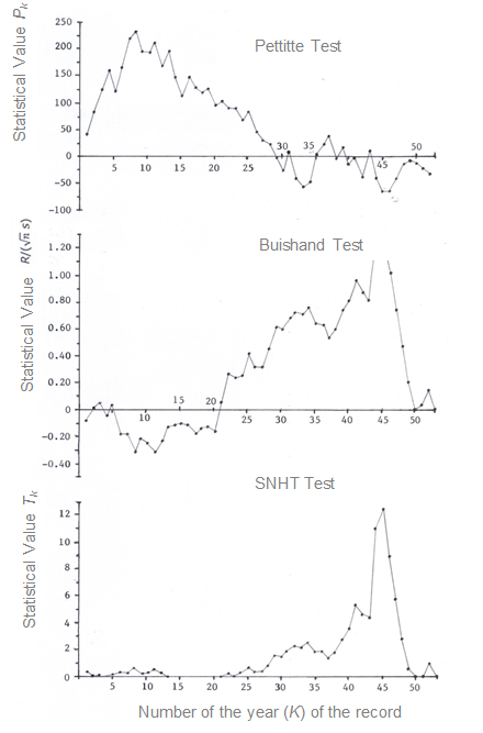
Figure 3 Graphs of the indicated statistical tests applied to the annual precipitation record of the Moctezuma station of the Potosino Plateau, Mexico
On the other hand, Figure 4 shows the graphs of the Pettitt, Buishand and SNHT tests, applied to the record of the El Mezquite station. The first two define maximum positive and negative extreme values and the third a single positive maximum, in k = 37 (year 2000). Accepting such year as a break point, a period from 2000 to 2016 is defined with 17 values and a mean of 579.365 mm after the change and 36 data and a mean of 327.811 mm before the change. With equation 10 a value of 1.7674 is obtained as the correction factor (f).
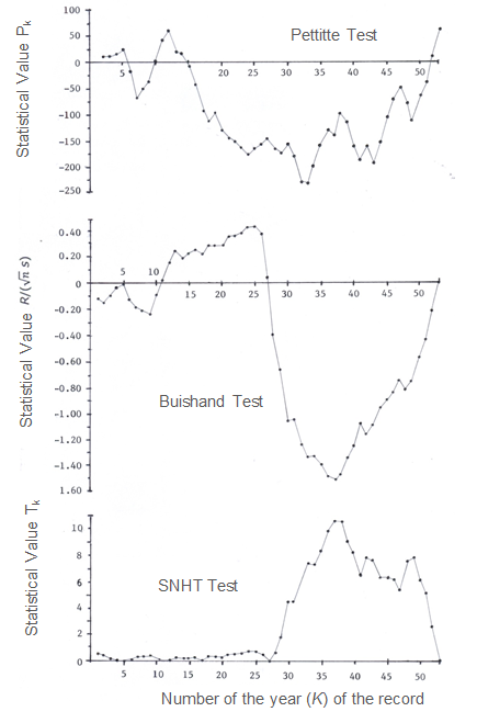
Figure 4 Graphs of the indicated statistical tests applied to the annual precipitation record of the El Mezquite station of the Potosino Plateau, Mexico.
In the corrected record of the El Mezquite station it has the following
statistical parameters: minimum = 59.9 mm; maximum = 1344.1 mm;
Conclusions
The exposed approach (Figure 2) when processing the climatic information of a geographical area allows working with similar magnitudes and when establishing a common period, such data must also show a similar behavior. The above can be seen in the values and statistical parameters set out in Table 2 and Table 3, relative to the 16 large records of annual precipitation processed from the Potosino Plateau of Mexico.
The results of this study can be specified in the following: it was found that 11 records are reliable, that is, homogeneous, three are less reliable (Vanegas, Palo Blanco and Villa de Arriaga) and two are unreliable (Moctezuma and El Mezquite). The first three non-homogeneous records owe their inconsistency to persistence; since they have significant serial correlation coefficients of order one (r 1).
Regarding the unreliable record of the Moctezuma station, the graphs of their Pettitt and Buishand tests (Figure 3) show a different behavior, without coincidence of the maximum, making it clear that there is no break point. On the contrary, the graphics of the El Mezquite station (Figure 4), with the Buishand and SNHT tests tend to define a maximum in the year 2000 (k = 37). By correcting the data before the change, a less reliable record is obtained.
Pettitt test is not considered sufficiently powerful or efficient, since it showed no loss of homogeneity in any of the five non-homogeneous records, which were detected by the other three applied tests. The above, in annual precipitation records of the semi-arid zone of the state of San Luis Potosí, Mexico.
Acknowledgments
Suggestions and recommendations of the two anonymous referees B and C are welcome, which allowed improving the description of the approach presented to prove loss of homogeneity in climatological records, due to non-climatic alterations. Figure 2 was included at the suggestion of referee B and the analysis of the non-homogeneous records, based on the results of the Pettitt, Buishand and SNHT tests, was formulated at the recommendation of both referees.
REFERENCES
Alexandersson, H. (1986). A homogeneity test applied to precipitation data. Journal of Climatology, 6(6), 661-675. [ Links ]
Alexandersson, H., & Moberg, A. (1997). Homogenization of Swedish temperature data. Part I: Homogeneity test for linear trends. International Journal of Climatology, 17(1), 25-34. [ Links ]
Beaulieu, C., Ouarda, T. B. M. J., & Seidou, O. (2007). Synthése des techniques d’homogénéisation des séries climatiques et analyse d’applicabilité aux series de precipitations. Hydrological Sciences Journal, 52(1), 18-37. [ Links ]
Beaulieu, C., Seidou, O., Ouarda, T. B. M. J., Zhang, X., Boulet, G., & Yagouti, A. (2008). Intercomparison of homogenization techniques for precipitation data. Water Resources Research, 44(2), W02425. [ Links ]
Buishand, T. A. (1982). Some methods for testing the homogeneity of rainfall records. Journal of Hydrology, 58(1-2), 11-27. [ Links ]
Campos-Aranda, D. F. (2005). FDP Gamma Mixta (Anexo B). En: Agroclimatología Cuantitativa de Cultivos (pp. 267-281). México, DF, México: Editorial Trillas. [ Links ]
Campos-Aranda, D. F. (2013). Caracterización de sequías meteorológicas mediante curvas de severidad-área-frecuencia, en el valle de San Luis Potosí, México. Tecnología y ciencias del agua, 4(3), 165-186. [ Links ]
Campos-Aranda, D. F. (2015). Búsqueda del cambio climático en la temperatura máxima de mayo en 16 estaciones climatológicas del estado de Zacatecas, México. Tecnología y ciencias del agua, 6(3), 143-160. [ Links ]
Dhorde, A. G., & Zarenistanak, M. (2013). Three-way approach to test data homogeneity: An analysis of temperatures and precipitation series over southwestern Islamic Republic of Iran. Journal of Indian Geophysical Union, 17(3), 233-242. [ Links ]
Ducré-Robitaille, J. F., Vincent, L. A., & Boulet, G. (2003). Comparison of techniques for detection of discontinuities in temperature series. International Journal of Climatology, 23(9), 1087-1101. [ Links ]
Eischeid, J. K., Baker, C. B., Karl, T. R., & Diaz, H. F. (1995). The quality control of long-term climatological data using objective data analysis. Journal of Applied Meteorology, 34(12), 2787-2795. [ Links ]
Guajardo-Panes, R. A., Granados-Ramírez, G. R., Sánchez-Cohen, I., Díaz-Padilla, G., & Barbosa-Moreno, F. (2017). Validación espacial de datos climatológicos y pruebas de homogeneidad: caso Veracruz, México. Tecnología y ciencias del agua, 8(5), 157-177. [ Links ]
Guijarro, J. A. (2014). Chapter 24. Quality control and homogenization of climatological series. In: Eslamian, S. (ed.). Handbook of Engineering Hydrology. Fundamentals and Applications (pp. 501-513). Boca Raton, USA: CRC Press. [ Links ]
González-Rouco, J. F., Jiménez, J. L., Quesada, V., & Valero, F. (2001). Quality control and homogeneity of precipitation data in the southwest of Europe. Journal of Climate, 14(5), 964-978. [ Links ]
Hanssen-Bauer, I., & Forland, E. J. (1994). Homogenizing long Norwegian precipitation series. Journal of Climate, 7(6), 1001-1013. [ Links ]
Khaliq, M. N., & Ouarda, T. B. M. J. (2007). On the critical values of the standard normal homogeneity test (SNHT). International Journal of Climatology, 27(5), 681-687. [ Links ]
Lanzante, J. R. (1996). Resistant, robust and non-parametric techniques for the analysis of climate data: Theory and examples, including applications to historical radiosonde station data. International Journal of Climatology, 16(11), 1197-1226. [ Links ]
Linsley, R. K., Kohler, M. A., & Paulhus, J. L. (1988). Chapter 14. Stochastic hydrology. In: Hydrology for Engineers (pp. 374-397). London, England: McGraw-Hill Book Co., SI Metric edition. [ Links ]
Machiwal, D., & Jha, M. K. (2012). Chapter 34. Methods for testing normality of hydrologic time series and methods for time series analysis (pp. 32-84). In: Hydrologic time series analysis: Theory and practice. Dordrecht, The Netherlands: Springer. [ Links ]
Mallakpour, I., & Villarini, G. (2016). A simulation study to examine the sensitivity of the Pettitt test to detect abrupt changes in mean. Hydrological Sciences Journal, 61(2), 245-254. [ Links ]
Mishra, A. K., & Singh, V. P. (2008). Chapter 23. Development of drought SAF curves. In: Singh, V. P. (ed.). Hydrology and Hydraulics (pp. 811-833). Highlands Ranch, Colorado, USA: Water Resources Publications. [ Links ]
Moberg, A., & Alexandersson, H. (1997). Homogenization of Swedish temperature data. Part II: Homogenized gridded air temperature compared with a subset of global gridded air temperature since 1861. International Journal of Climatology, 17(1), 35-54. [ Links ]
Paulhus, J. L. M., & Kohler, M. A. (1952). Interpolation of missing precipitation records. Monthly Weather Review, 80(8), 129-133. [ Links ]
Peterson, T. C., Easterling, D. R., Karl, T. R., Groisman, P., Nichols, N., Plummer, N., Torok, S., Auer, I., Boehm, R., Gullett, D., Vincent, L., Heino, R., Tuomenvirta, H., Mestre, O., Szentimrey, T., Salinger, J., Førland, E. J., Hanssen‐Bauer, I., Alexandersson, H., Jones, P., & Parker, D. (1998). Homogeneity adjustments of in situ atmospheric climate data: a review. International Journal of Climatology, 18(13), 1493-1517. [ Links ]
Pettitt, A. N. (1979). A non-parametric approach to the change-point problem. Applied Statistics, 28(2), 126-135. [ Links ]
Rhoades, D. A., & Salinger, M. J. (1993). Adjustment of temperature and rainfall records for site changes. International Journal of Climatology, 13(8), 899-913. [ Links ]
SARH, Secretaría de Agricultura y Recursos Hidráulicos. (1980). Boletín Climatológico No. 3. Región Hidrológica No. 37 (El Salado). México, DF, México: Secretaría de Agricultura y Recursos Hidráulicos. Subsecretaría de Planeación, Dirección General de Estudios, Subdirección de Hidrología. [ Links ]
Shapiro, S. S., & Wilk, M. B. (1965). An analysis of Variance Test for Normality (Complete Samples). Biometrika, 52(3-4), 591-611. [ Links ]
Shapiro, S. S. (1998). Chapter 6. Selection, fitting and testing statistical models. In: Wadsworth, H. M. (ed.). Handbook of statistical methods for engineers and scientists, 2nd ed. (pp. 6.1-6.35). New York, USA: McGraw-Hill Inc. [ Links ]
Syrakova, M. & Stefanova, M. (2009). Homogenization of Bulgarian temperature series. International Journal of Climatology, 29(12), 1835-1849. [ Links ]
Toreti, A., Kuglitsch, F. G., Xoplaki, E., Della-Marta, P. M., Aguilar, E., Prohom, M., & Luterbacher, J. (2011). A note on the use of the standard normal homogeneity test to detect inhomogeneity in climatic time series. International Journal of Climatology, 31(4), 630-632. [ Links ]
Tuomenvirta, H. (2001). Homogeneity adjustments of temperature and precipitation series-Finnish and Nordic data. International Journal of Climatology, 21(4), 495-506. [ Links ]
Wijngaard, J. B., Klein-Tank, A. M. G., & Können, G. P. (2003). Homogeneity of 20th century European daily temperature and precipitation series. International Journal of Climatology, 23(6), 679-692. [ Links ]
WMO, World Meteorological Organization. (1971). Annexed III: Standard tests of significance to be recommended in routine analysis of climatic fluctuations. In: Climatic change (pp. 58-71) (Technical Note No. 79). Geneva, Switzerland: World Meteorological Organization. [ Links ]
Young, K. C. (1992). A three-way model for interpolating for monthly precipitation values. Monthly Weather Review, 120(11), 2561-2569. [ Links ]
Yozgatligil, C., & Yazici, C. (2016). Comparison of homogeneity tests for temperature using a simulation study. International Journal of Climatology, 36(1), 62-81. [ Links ]
Received: October 09, 2018; Accepted: October 22, 2019
 Este es un artículo publicado en acceso abierto bajo una licencia
Creative Commons
Este es un artículo publicado en acceso abierto bajo una licencia
Creative Commons
