


Servicios Personalizados
Revista
Articulo
 texto en
  Inglés (pdf)
 Artículo en XML
 Referencias del artículo
 Enviar artículo por email
Indicadores
-
 Citado por SciELO
 -
 Accesos
Links relacionados
-
 Similares en
SciELO
Similares en
SciELO
Compartir

 Permalink
Tecnología y ciencias del agua
versión On-line ISSN 2007-2422
Tecnol. cienc. agua vol.11 no.5 Jiutepec sep./oct. 2020 Epub 10-Jun-2024
https://doi.org/10.24850/j-tyca-2020-05-09
Articles
Distributed hydrologic model using GPM-IMERG images in the Huaynamota River Watershed, Nayarit, México
1
 http://orcid.org/0000-0003-0392-6004
2
http://orcid.org/0000-0001-9287-655X
1Universidad Autónoma Chapingo, Texcoco, México, alberto.espinosa.74@gmail.com
2Universidad Autónoma Chapingo, Texcoco, México, libacas@gmail.com
3Universidad Autónoma Chapingo, Texcoco, México, arteagar@correo.chapingo.mx
4Centro de Investigación en Geografía y Geomática “Ing. Jorge L. Tamayo”, Centro de Investigación en Ciencias de Información Espacial A. C. del Consejo Nacional de Ciencia y Tecnología, Ciudad de México, México, geomauricio23@gmail.com
In Mexico, it is necessary to exploit water resources to cover different needs and to control them to prevent damage caused by extreme events. The objective of this study was to model and calibrate hydrographs calculated with rainfall data measured with GPM-IMERG satellite images in the Huaynamota River watershed and compare the results with a hydrological model fed rainfall data from automated meteorological stations. The research was conducted in a tributary of the Huaynamota River, which is part of the Lerma-Chapala-Santiago hydrological region. The watershed is located in the states of Zacatecas, Durango, Jalisco and Nayarit. For analysis of the hydrographs at the basin outlet, maximum rainfall events occurring in the periods July 21 to 26, 2016, August 14 to 24, 2017, and September 1 to 16, 2017, were evaluated. The model was developed in HEC-HMS, using methods such as the runoff curve number and the Clark unit hydrograph. Comparison of the measured and simulated hydrographs showed good fit of the simulation with reality. In most of the modeled events, the Nash-Sutcliffe coefficient was above 0.5, which is considered acceptable. We concluded that hydrological modeling using satellite meteorological images is a good option that can be implemented in regions where hourly rainfall data gauged with land instruments are not available.
Keywords: Rainfall GPM-IMERG satellite images; Clark unit hydrograph; distributed model; lumped model
En México es necesaria la explotación y el control de los recursos hídricos, ya sea para cubrir las diversas carestías o para protegerse del daño causado por eventos extremos. Esta investigación tuvo como objetivo modelar y calibrar los hidrogramas de una cuenca, calculados con datos de lluvia y medidos con imágenes de satélite GPM-IMERG en la cuenca del río Huaynamota, México, así como comparar los resultados con un modelo hidrológico alimentado con datos de lluvia de estaciones meteorológicas automáticas. Esta investigación se realizó en un tributario de la cuenca del río Huaynamota, el cual es parte de la región hidrológica Lerma-Chapala-Santiago. La cuenca se ubica en los estados de Zacatecas, Durango, Jalisco y Nayarit. Para el análisis de los hidrogramas a la salida de la cuenca se evaluaron eventos de lluvia máximos ocurridos en los periodos del 21 al 26 de julio de 2016, del 14 al 24 de agosto de 2017, y del 1° al 16 de septiembre de 2017. El modelo se desarrolló en HEC-HMS, con base en métodos como el número de curva de escurrimiento y el hidrograma unitario de Clark. La comparación de los hidrogramas medidos y aparentados mostró un buen ajuste de lo simulado con la realidad. En la mayoría de los eventos modelados, el coeficiente de Nash-Sutcliffe fue mayor a 0.5, que se considera aceptable. Se concluyó que la modelación hidrológica a partir de imágenes de satélites meteorológicos es una buena opción para su implementación en regiones donde se carece de datos de lluvia horaria medida con instrumentos en tierra.
Palabras clave: imagen de satélite para lluvia GPM-IMERG; hidrograma unitario de Clark; modelo distribuido; modelo agregado
Introduction
Understanding the physical behavior of storms is of great importance for the solution of diverse problems associated with precipitation, such as floods, weather prediction, agriculture, cloud physics, etc. (Ioannidou, Kalogiros, & Stavrakis, 2016). The scarcity of hourly rainfall data is a problem faced by hydrologists in modeling watersheds for prediction purposes. Reliability of the results of modeling depends largely on the availability of meteorological information: hydrometric information to calibrate and validate a hydrological model (Magaña-Hernández, Ba, & Guerra-Cobián, 2013. Moreover, temporal and spatial data must be sufficient since, if these required data are hourly and if there are requirements in terms of spatial distribution, the complexity increases.
Méndez-Antonio et al. (2013) point out that technologies such as radar and weather satellites are capable of estimating spatial variability of precipitation in real time and can be very useful in hydrological modeling. With GIS (Geographic Information System) applications, it is possible to generate information with very little temporal variability at the moment the event occurs.
With advances in computational systems and launching of different space missions, a wide variety of products have been developed to monitor physical changes in the atmosphere and the earth’s surface. This has permitted important developments in different areas of tele-detection (Olivera & Maidment, 1999).
Rainfall data from satellite images are uniformly distributed in space. This makes them an alternative for hydrological modeling (Zubieta, Getirana, Espinoza, Lavado-Casimiro, & Aragon, 2017).
These products reduce the limitations often faced in terms of availability and acquisition of data, making it possible to implement distributed models, which consider spatial variability of the physical characteristics of the watershed and of rainfall and divide the watershed into subbasins or cells (Méndez-Antonio, Soto-Cortés, Rivera-Trejo, & Caetano, 2014).
According to Mendez Antonio et al. (2014), one of the advantages of these models is that they permit analysis of different elements that affect hydrological response, such as vegetation and land use. These elements make it possible to obtain flows at different points of the watershed. This is possible since spatial variation of precipitation, infiltration, losses and runoff are explicitly considered, while in lumped models these variations are averaged or ignored.
Lumped models, according to Vieux (2004), have some disadvantages. a) Deriving parameters at the sub-basin scale is complicated because runoff is not available at each outlet. b) Precision of the calculation of flows is affected by the number of sub-basins. c) Variations of the properties in the sub-basins are ignored or averaged.
The objective of this study was to simulate the flows in the Huaynamota River watershed, Mexico, using the modified Clark Unit Hydrograph method (ModClark) integrated in HEC-HMS fed with precipitation data estimated from Global Precipitation Measurement GPM (IMERG) satellite images and to calibrate and validate the model. In the following section, details of the options used in this study to calculate HEC-HMS will be explained.
Materials and methods
Study area
The Huaynamota River watershed ―up to the Chapalagana hydrometric station― forms part of the Lerma-Chapala-Santiago hydrological region 12, which includes parts of the states of Zacatecas, Durango, Nayarit and Jalisco. It is located between 104° 35’ and 103° 20’ W and between 23° 25’ and 21° 23’ N. The watershed covers an area of 12 080 km2 to the gauging station Chapalagana (Figure 1). The study area is bounded by the watershed of the Atengo River (also known as the Chapalagana River), a tributary of the Huaynamota River. The Huaynamota River has two main tributaries: the Jesús María and the Atengo Rivers. Downstream, the Huaynamota River joins the Santiago River which flows into the Pacific Ocean at the town of Santiago Ixcuintla, Nayarit. The watershed was delimited with HEC-GeoHMS 10.1 (in the ArcMap 10.3 platform) using the digital elevation model (INEGI, 2017c), with a resolution of 15 m; the range of elevations is 2500 to 220 m. The mean slope of the watershed is 28%, the river slope is 0.68% and concentration time is 38 hours. Average yearly rainfall is 600 mm, concentrated in the period from July to October. The watershed contributes runoff to the Aguamilpa reservoir located approximately 29 km downstream from the Chapalagana gauging station, which is the outlet of the watershed under study.

Sources of information
GPM (IMERG) GIS images are available free at https://pmm.nasa.gov/data-access/downloads/gpm. These images have a spatial resolution of 0.1° x 0.1° with a temporality of 30 min (Huffman et al., 2017).
The hourly hydrometric data from the Chapalagana station and of precipitation from the Automated Meterological Stations (AMS) (Table 1) were obtained from the Comisión Federal de Electricidad (CFE, 2018).
Table 1 Automated Meteorological Stations in the Huaynamota River watershed up to the Chapalagana station.
| Administrator | Name | Longitude | Latitude |
|---|---|---|---|
| CFE | Florida | -103.6036° | 22.6864° |
| CFE | Platanitos | -104.063° | 22.5680° |
| CFE | Bolaños | -103.7833° | 21.8250° |
| CFE | Jesús María | -104.5160° | 22.2550° |
| CFE | Chapalagana | -104.5080° | 21.9450° |
To construct the digital map raster that shows spatial variation of the runoff curve number (CN), we used a set of vectoral data of land use and vegetation of the Instituto Nacional de Estadística y Geografía (INEGI), scale 1:250,000 series V, 2011-2012 (INEGI, 2017a) and the set of edaphological vectoral data scale 1:250,000 series II, 2002-2007 (INEGI, 2017b).
Procedure
The runoff production function derived from the runoff curve number method (CN) of the Soil Conservation Service of the Department of Agriculture of the United States is one of the most used methods because of its simplicity in estimating excess precipitation as a function of accumulated precipitation, soil type, vegetation and antecedent moisture (Ponce & Hawkins, 1996).
The procedure is based on the water balance equation and on two fundamental hypotheses, according to Sithara (2015). The first establishes that the ratio between direct runoff volume and maximum potential runoff on an impermeable surface is equal to the ratio between real infiltration and maximum potential infiltration. The second hypothesis establishes that initial infiltration is a fraction of potential retention. Equations (1), (2) and (3) represent this pair of hypotheses:
where Q = direct runoff or effective precipitation (mm); P = total precipitation (mm); I a = Initial abstractions (mm); F = accumulated infiltration excluding I a ; S = retention or maximum potential infiltration (mm). For practical application, I a = 0.2 S.
As initial abstractions, five categories are considered (Ponce & Hawkin, 1996): (1) interception by vegetation foliage; (2) interception in reservoirs; (3) infiltration into subsoil; (4) evaporation from bodies of water and soil, and (5) evapotranspiration of the vegetation.
Combining Equation (1) and Equation (2), we have:
Substituting I a = 0.2 S in Equation (4):
where Q = 0 for P ≤ 0.2 S, and S in terms of CN is represented with Equation (6):
where CN = runoff curve number. To illustrate the variation range of CN values, CN=98 represents an impermeable surface, and CN=30 is for permeable soils with high rates of infiltration (USACE, 2000).
The function of runoff transfer is performed with the modified Clark unit hydrograph method. According to Kull and Feldman (1998), the method consists of routing the runoff produced in each cell to the outlet of the watershed after a lapse of time equal to the run time from the cell to the outlet (Equation 7):
where t cell is the travel time of the cell in hours, t c is the concentration time of the watershed in hours, d cell is the travel distance from a cell to the watershed outlet in meters, and d max is the distance from the farthest cell to the outlet. The results of each cell are combined to produce the final hydrograph, as shown conceptually in Figure 2.

To calculate the produced hydrograph of the watershed, the ModClark method requires estimation of the parameters concentration time (tc) and reservoir coefficient (R).
According to McCuen, Wong and Rawls (1984), there are two accepted definitions of concentration time (tc). The first defines tc as the time a drop of water requires to arrive at the farthest point of the watershed, its outlet. The second is based on the hyetograph of the storm and the hydrograph, while concentration time is the time between the center of the excess rain mass and the point of inflection in the recession of the hydrograph of direct runoff. We used the equation of Kirpich expressed in equation (8) (Chow, Maidment, & Mays, 1988):
where t c is the concentration time in h; L is the length of the main channel of the watershed in m, and S is the slope of the main channel (m/m).
The reservoir coefficient is estimated from an observed hydrograph. It represents the ratio between the low volume of the hydrograph after the second inflection point (recession curve) and the value of the flow at this point (USACE, 1982). Equation (9) estimates this coefficient:
where R is the storage coefficient;
Domínguez et al. (2008) point out that c can be equal to 0.6, but the US Army Corps of Engineers, cited by Magaña-Hernández et al. (2013), recommends that c should be equal to 0.8. In our study, it was calculated with 0.75·t c , since this value generated the best results in the calibration process.
Runoff routing was calculated with the Muskingum method using the following equation:
Equation (11) relates storage (S), inputs (I) and outputs (O) of the analyzed section (Bedient, Huber, & Vieux, 2013), where S is the storage in the section of the current; I is the input flow; O is the output flow; K is a constant of time the current takes to pass through the section; x is a weight factor that relates inputs and outputs of the storage of the section of current.
To evaluate the model, we used two measures: the Nash-Sutcliffe efficiency coefficient, NSE (Nash & Sutcliffe, 1970), and the root square mean of the error (RSME) (Vargas-Castañeda, Ibáñez-Castillo, & Arteaga-Ramírez, 2015):
where Y obs is the observed value, Y sim is the simulated value, Y mean is the mean of the observed data.
The coefficient of NSE evaluates the magnitude of residual variance between observed and modeled data (Equation 12). The coefficient varies from -∞ to 1. NSE = 1 is the optimal value, between 0 and 1 is acceptable, while for values ≤ 0 the mean is considered a better predictor than the simulated value and thus model performance is considered inacceptable. Moriasi et al. (2007) propose the NSE ranges presented in Table 2.
Table 2 Criteria for evaluation of hydrologic models using the Nash-Sutcliffe efficiency index (NSE).
| Interval | Classification |
|---|---|
| NSE < 0.5 | Unsatisfactory |
| 0.5 < NSE < 0.65 | Satisfactory |
| 0.65 < NSE < 0.75 | Good |
| 0.75 < NSE < 1.0 | Very good |
The coefficient RSME (Equation (13)) measures the mean error, in absolute terms, between observed and simulated data and has the hydrograph units of the flows, which are compared: in this case m3/s.
To implement the model, the following was necessary:
Physiographic characteristics were determined (Figure 3) using a digital model of elevation (MDE) downloaded from Continuo de Elevaciones Mexicano 3.0 (CEM 3.0), which has a resolution of 15 m. This delimited the watershed and sub-basins, identified the main channel, and provided physiographic parameters, with the HEC-GeoHMS extension, which is distributed free by USACE (2013) for ArcMap 10.3.

Spatial variation of the runoff curve number, CN (Figure 4), was determined with the vectoral edaphology layers of series II and land use and vegetation series V of INEGI (2017a), with the procedure proposed by USACE (2013) in HEC-GeoHMS for ArcMap 10.3.
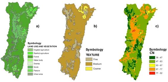
Figure 4 a) Land use and vegetation; b) texture type; c). curve number in the Huaynamota River watershed.
The process of calibrating the hydrological model in HEC-HMS version 4.2
Observed flows can be used to optimize model functioning by estimating or improving parameter values. The process of optimization begins with initial parameter values, and these parameters are adjusted so that simulated results approximate observed flows as closely as possible. HEC-HMS version 4.2 uses two search algorithms of the parameters that minimize this difference, or error. These algorithms begin with the initial value they are given and continue until they find the optimal value. The objective of this search algorithm is to minimize the difference between observed and simulated values. If the observed and simulated hydrographs were totally identical, this error or difference, would be zero.
Search algorithm: The two search algorithms that HEC-HMS version 4.2 can use are the univariate gradient method and the Nelder and Mean method (USACE, 2015). The univariate gradient method evaluates and fits a parameter, while the rest are left constant. The Nelder and Mead method uses a simplex algorithm to evaluate all the parameters simultaneously and determines which parameter to adjust. HEC-HMS uses the univariate gradient method by default.
Objective function: The objective function measures the goodness of fit between calculated and observed flows. HEC-HMS 4.2 gives the option of selecting among eight different objective functions (USACE, 2015): (1) RMSE error function, calculates the root mean square error; (2) the weighted RMSE error function is like the previous objective function, but it gives more weight to flows that are above the mean and less weight to flows that are below the mean; the HEC-HMS user manual does not give details of how much it is weighted; (3) RMSE error function is applied to flow logarithms to emphasize the differences between small and large flows; (4) the function SSR, sum of square residuals, gives greater weight to large errors than to small errors; (5) the absolute sum of residuals function gives equal weight to large and small errors; (6) the function of error percentage in the maximum flow only emphasizes this value; (7) the function volume error ignores maximum flows or the considerations of the real moment in which the flows occur, in favor of considering optimizing volume; (8) the function occurrence time gives greater emphasis to errors that occur at the end and less to those that occur at the beginning, favoring a “warm-up” stage for the model. By default, HEC-HMS selects function #2, which gives more importance to not erring when calculating flows that are above the mean.
Calibration of this model: This study was conducted in HEC-HMS version 4.2. The univariate gradient model was used as a search algorithm to find the optimal value, and the objective function considered was that that most penalized mistakes in calculating a flow above the mean. The latter was selected because we expected this model to be useful in predicting floods to enable alerting the populations, and the threat is greater with flows above the mean. The HEC-HMS model reports the root square mean of the error (RSME) and the Nash-Sutcliffe (NS) coefficient as coefficients of fit. The user has the option of automatically giving HMS groups of parameters to be optimized, for example, all the runoff curve numbers by sub-basin, or the delay times or concentration times, or all the parameters of channel routing, etc. Another option would be adding parameters and, by trial and error, see how sensitive the objective function is to these changes. In our study, we did several tests, by trial and error, adding parameters to determine how sensitive the optimization process was since HEC-HMS, for each optimized parameter, reports what it calls “objective function sensitivity”. The literature reports that, of the superficial hydrological models, one of the most sensitive parameters is the runoff curve number (Moriasi et al., 2007), and this can be demonstrated. However, we began from a CN value obtained from soil type and vegetation cover; it permitted this parameter to vary only up to ± 20% when calibrating. The other parameter that was found to be sensitive was the storage coefficient R (Equation (10)), which is c times the concentration time. Values between 0.6 and 0.75 were tested, as reported in the literature (Domínguez et al., 2008; Magaña-Hernández et al., 2013). There was better response when the value of c was 0.75. Flood channel routing parameters were tested with Muskingum, K and x, but there was no notable improvement in reducing the error between observed and simulated flows. We did not select the automatic mode of HEC-HMS calibration because it arbitrarily modifies hydrological parameters notably to force the fit between observed and simulated data.
Three final summarized comments regarding procedure:
Two hydrological models were run in the environment of HEC-HMS version 4.2: (1) a hydrological model lumped with the Original Clark UH with hourly meteorological information from the CFE automated meteorological stations (AMS), (2) a hydrological model distributed with the Modified Clark UH, with hourly meteorological information derived from GPM-IMERG satellite images. Both models used the runoff curve number methodology to calculate runoff depths, and both models routed channel floods with the Muskingum method.
In the construction of the rainfall database from satellite images, a time series was generated with GPM-IMERG images for each selected event. Image pre-processing was carried out in ArcMap to later convert them to *.dss format with the tool asc2dssGrid.exe (USACE, 2016) included in the HEC-GeoHMS extension.
The rainfall events considered in the modeling were three: (1) July 21 to 26, 2016; (2) August 14 to 24, 2017; and (3) September 1 to 16, 2017. During these periods, rainfall data from GPM-IMERG satellite images and hourly rainfall and flow data from the CFE AMS were available.
Results
Table 3 shows the results of the hydrological models executed with information from CFE weather stations and with rainfall data from satellite images. In Table 3, the best results were obtained from those hydrological models fed directly with rainfall data registered by the CFE AMS. The fit of hydrological models fed rainfall data estimated from satellite images was poor, as measured with the Nash-Sutcliffe (NSE) efficiency index and with the root square mean of the error (RSME). It is likely that the data from images had not been calibrated by NASA with temporal and spatial information as detailed as that of the CFE. But it is worth mentioning that data from the CFE, unlike the Servicio Meteorológico Nacional (SMN), is not open to the public. However, in Mexico, in places were data from CFE or SMN automated weather stations do not exist or are not distributed spatially as desired, the NASA images are a good alternative for development of hydrological models. Moreover, of the three events modeled in this study, only that of July 21 to 26, 2016, had poor fit, as measured with NSE efficiency index and with RSME.
Table 3 Results of the calibrated hydrological models.
| Date of the event | Source of rainfall data | Qcalc (m3 s-1) | Qobs (m3 s-1) | Vcalc (mm) | Vobs (mm) | RSME (m3 s-1) | NSE |
|---|---|---|---|---|---|---|---|
| 21-26 July 2016 | AMS | 440.2 | 641.9 | 4.52 | 3.73 | 73.0 | 0.625 |
| Satellite images | 373.6 | 641.9 | 3.33 | 3.73 | 129.3 | -0.159 | |
| 14-24 August 2017 | AMS | 439.5 | 465.9 | 5.06 | 5.18 | 23.0 | 0.932 |
| Satellite images | 462.0 | 465.9 | 6.26 | 5.18 | 60.5 | 0.531 | |
| 1-16 September 2017 | AMS | 624.7 | 1171.0 | 32.44 | 35.22 | 186.7 | 0.567 |
| (Longest event of 2017) | Satellite images | 969.4 | 1171.0 | 44.16 | 35.22 | 194.3 | 0.530 |
Figure 5 shows the processed rainfall data from satellite images for the June 21 to 26, 2016, event, and Figure 6 shows the model runs with AMS data and with data from satellite images. Regarding maximum flows, it can be observed that the model fed AMS data obtains better results in predicting both value and the hour it occurred.
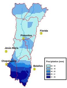
Figure 5 Accumulated precipitation, data from GPM-IMERG images for the event of July 21 to 26, 2016.
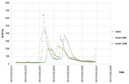
Figure 6 Observed and simulated flows at the Chapalangana station for the events that occurred from July 21 to 26, 2016.
Figure 7 shows processed rainfall data from satellite images for August 14 to 24, 2017, and Figure 8 shows the model runs with both AMS data and data from satellite images. In terms of maximum flows, the model fed AMS data resulted in better and very good results (NSE=0.932). The observed hydrograph can almost be superimposed onto the hydrograph simulated with AMS data (Figure 8). The model fed satellite image data ran very well until a two-day period, between August 19 and 21, decreased its fit to an NSE of 0.531. The AMS model is almost perfect with respect to flow values and volumes and in terms of temporal prediction of flows.
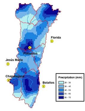
Figure 7 Accumulated precipitation. Data from GPM-IMERG images for the event that occurred August 14 to 24, 2017.
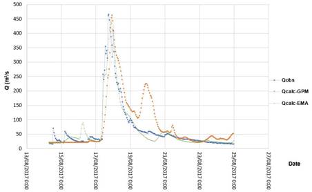
Figure 8 Observed and simulated flows at the Chapalagana station for the event that occurred August 14 to 24, 2017.
Figure 9 shows the processed rainfall data from satellite images for September 1 to 16, 2017, and Figure 10 shows the model runs with AMS data and satellite image data. With respect to maximum flows, the model fed AMS data obtained the better results, with NSE = 0.567., while the model fed data from images has an NSE of 0.530. It should be noted that, although the AMS model, measured with NSE and RSME, is slightly superior, the model fed rainfall data from images had an error of 17% in estimating maximum flow, while the model with AMS data had an error of approximately 50%. In terms of volumes, the model fed AMS data also had better results.
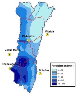
Figure 9 Accumulated precipitation. Data from GPM-IMERG images for the event that occurred September 1 to 16, 2017.
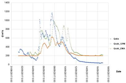
Figure 10 Observed and simulated flows at the Chapalagana station for the event of September 1 to 16, 2017.
If this work is compared with other previous studies conducted in Mexico, the comparison perhaps pertains to radar rainfall data. In the models fed by radar, the size of the watershed varies from 35 to 3 242 km2 (Magaña-Hernández et al., 2013; Méndez-Antonio et al., 2014), while in our study we have a watershed of approximately 12 000 km2, making instrumentation and representation of spatial rainfall distribution more difficult.
There are two relatively recent studies of hydrological models with satellite images (Zubieta et al., 2017; Zubieta, Laqui, & Lavado, 2018). Both studies use satellite images for rainfall, but one of the studies is at a daily time scale and the other is monthly. Our study is at an hourly scale.
Discussion
The Nash-Sutcliffe is observed to be more efficient in all of the events simulated with lumped models using the Clark Unit Hydrograph, which was supplied with precipitation data from five stations distributed over the Huaynamota River watershed’s area of 12,075 km2, even though it did not represent uniform spatial rainfall distribution.
This may have two reasons: (1) the flow velocity between cells was considered constant, affecting the parameters concentration time and storage coefficient; cell size for each of the grids used in the study was 2 km x 2 km; (2) data measured on land are definitively more reliable than image data. However, the NASA’s GMP-IMERG satellite images are a good option where there is no land meteorological information with sufficient spatial and temporal (hourly) distribution.
Conclusions
The rainfall data recorded by the automatic meteorological stations (AMS), compared to those of the satellite images GPM-IMERG, represented better the rainfall-runoff process.
Because precipitation is the main input for hydrological modeling, the use of this new generation of images is of great interest in hydrological studies. However, future studies should consider calibration of the images with precipitation information from stations located in national territory.
It is concluded from the results of hydrological modeling with rainfall data estimated from images and compared with the model with data from AMS that satellite images are a good option for hydrological modeling, applicable where meteorological information measured on land is deficient.
Acknowledgements
Our thanks to the Comisión Federal de Electricidad for allowing access to their hydrometeorological database through their website administered by the Instituto Nacional de Electricidad y Energías Limpias.
REFERENCES
Bedient, P. B., Huber, W. C., & Vieux, B. E. (2013). Hydrology and floodplain analysis (5th ed.). New York, USA: Pearson. [ Links ]
Chow, V. T., Maidment, D. R., & Mays, L. W. (1988). Applied hydrology. New York, USA: McGraw-Hill. [ Links ]
CFE, Comisión Federal de Electricidad. (2018). Sistema de Monitoreo de Cuencas de CFE. Recuperado de https://h06814.iie.org.mx/cuencas/logon.aspx?ReturnUrl=%2Fcuencas%2Fdefault.aspx [ Links ]
Domínguez, M. R., Esquivel, G. G., Méndez, A. B., Mendoza, R. A., Arganis, J. M. L., & Carrioza, E. E. (2008). Manual del modelo para pronóstico de escurrimiento. Ciudad de Mexico, México: Instituto de Ingeniería, Universidad Nacional Autónoma de México. Recuperado de https://doi.org/10.13140/RG.2.1.4687.5287 [ Links ]
Huffman, G. J., Bolvin, D. T., & Nelkin, E. J. (2017). Integrated multi-satellite retrievals for GPM (IMERG) Technical documentation. Purdue, USA: National Aeronautics and Space Administration. [ Links ]
INEGI, Instituto Nacional de Estadística y Geografía. (2017a). Conjunto de datos vectoriales de uso de suelo y vegetación. Serie V. Recuperado de https://www.inegi.org.mx/temas/usosuelo/ [ Links ]
INEGI, Instituto Nacional de Estadística y Geografía. (2017b). Conjunto de datos vectoriales edafológico. Serie II. Recuperado de https://www.inegi.org.mx/temas/edafologia/ [ Links ]
INEGI, Instituto Nacional de Estadística y Geografía. (2017c). Continuo de elevaciones mexicano 3.0 (CEM 3.0). Recuperado de https://www.inegi.org.mx/app/geo2/elevacionesmex/index.jsp [ Links ]
Ioannidou, M. P., Kalogiros, J. A., & Stavrakis, A. K. (2016). Comparison of the TRMM precipitation radar rainfall estimation with ground-based disdrometer and radar measurements in South Greece. Atmospheric Research, 181, 172-185. Recuperado de https://doi.org/10.1016/j.atmosres.2016.06.023 [ Links ]
Kull, D. W., & Feldman, A. D. (1998). Evolution of Clark’s unit graph method to spatially distributed runoff. Journal of Hydrologic Engineering, 3(1), 9-19. Recuperado de https://doi.org/10.1061/(ASCE)1084-0699(1998)3:1(9) [ Links ]
Magaña-Hernández, F., Ba, K. M., & Guerra-Cobián, V. H. (2013). Estimación del hidrograma de crecientes con modelacion determinística y precipitación derivada de radar. Agrociencia, 47(8), 739-752. [ Links ]
McCuen, R. H., Wong, S. L., & Rawls, W. J. (1984). Estimating urban time of concentration. Journal of Hydraulic Engineering, 110(7), 887-1002. Recuperado de https://doi.org/10.1061/(ASCE)0733-9429(1984)110:7(887) [ Links ]
Méndez-Antonio, B., Caetano, E., Soto-Cortés, G., Rivera-Trejo, F. G., Carvajal Rodríguez, R. A., & Watts, C. (2013). Weather radar data and distributed hydrological modelling: An application for Mexico Valley. Open Journal of Modern Hydrology, 3(2), 79-88. Recuperado de https://doi.org/10.4236/ojmh.2013.32011 [ Links ]
Méndez, A. B., Soto-Cortés, G., Rivera-Trejo, F., & Caetano, E. (2014). Modelación hidrológica distribuida apoyada en radares meteorológicos. Tecnología y ciencias del agua, 5(1), 83-101. [ Links ]
Moriasi, D. N., Arnold, J. G., Van Liew, M. W., Bingner, R. L., Harmel, R. D. & Veith, T. L. (2007). Model evaluation guidelines for systematic quantification of accuracy in watershed simulations. American Society of Agricultural and Biological Engineers, 50(3), 885-900. Recuperado de https://doi.org/10.13031/2013.23153 [ Links ]
Nash, J. E., & Sutcliffe, J. V. (1970). River forecasting trough conceptual models. Part 1 - A discussion of principles. Journal of Hydrology, 10(3), 282-290. Recuperado de https://www.sciencedirect.com/science/article/abs/pii/0022169470902556?via%3Dihub [ Links ]
Olivera, F., & Maidment, D. (1999). Geographic information systems (GIS)-based spatially dustributed model for runoff routing. Water Resources Research, 35(4), 1155-1164. Recuperado de https://www.researchgate.net/publication/228582442_Geographic_Information_Systems_GIS-Based_Spatially_Distributed_Model_for_Runoff_Routing [ Links ]
Ponce, V. M., & Hawkins, R. H. (1996). Runoff curve number: Has it reached maturity? Journal of Hydrologic Engineering, 1(1), 11-19. Recuperado de https://doi.org/10.1061/(ASCE)1084-0699(1996)1:1(11) [ Links ]
Sithara, J. (2015). GIS based Runoff estimation using NRCS method and time-area method. Scientific & Engineering Research, 5(7), 306-312. [ Links ]
USACE, United States Army Corps of Engineers. (1982). HEC-1 Training document No.15. California, USA: United States Army Corps of Engineers. [ Links ]
USACE, United States Army Corps of Engineers. (2000). Hydrologic Modeling System-HEC-HMS: Technical Reference Manual. Washington, DC, USA: United States Army Corps of Engineers. [ Links ]
USACE, United States Army Corps of Engineers. (2013). HEC-GeoHMS geospatial hydrologic modelling extension: user’s manual version 4.2. User’s manual-version 10.1. Recuperado de http://www.hec.usace.army.mil/software/hec-geohms/ [ Links ]
USACE, United States Army Corps of Engineers. (2015). HEC-HMS user’s manual version 4.1. Recuperado de http://www.hec.usace.army.mil/software/hec-hms/ [ Links ]
USACE, United States Army Corps of Engineers. (2016). Workshop: Application of HEC-HMS using gridded precipitation in watersheds outside of the United States. Recuperado de https://www.hec.usace.army.mil/training/CourseMaterials/Mongolia_Workshop/Workshop_Mongolia.pdf [ Links ]
Vargas-Castañeda, G., Ibáñez-Castillo, L. A., & Arteaga-Ramírez, R. (2015). Development, classification and trends in rainfall-runoff modeling.Ingeniería Agrícola y Biosistemas, 7(1), 5-21. Recuperado dehttp://dx.doi.org/10.5154/r.inagbi.2015.03.002 [ Links ]
Vieux, B. (2004). Distributed hydrologic modeling using GIS. Water Science and Technology Library. Book 48 (2nd ed.). New York, USA: Springer. [ Links ]
Zubieta, R., Getirana, A., Espinoza, J. C., Lavado-Casimiro, W., & Aragon, L. (2017). Hydrological modeling of the Peruvian-Ecuadorian Amazon Basin using GPM-IMERG satellite-based precipitation dataset. Hydrology and Earth System Sciences, 21(7), 3543-3555. Recuperado de https://doi.org/10.5194/hess-21-3543-2017 [ Links ]
Zubieta, R., Laqui, W., & Lavado, W. (2018). Modelación hidrológica de la cuenca del río Ilave a partir de datos de precipitación observada y de satélite, periodo 2011-2015, Puno, Perú. Tecnología y ciencias del agua, 9(5), 85-105. Recuperado de https://doi.org/10.24850/j-tyca-2018-05-04 [ Links ]
Received: February 07, 2019; Accepted: December 02, 2019
 Este es un artículo publicado en acceso abierto bajo una licencia
Creative Commons
Este es un artículo publicado en acceso abierto bajo una licencia
Creative Commons
