Flood frequency analysis

Planning, design, construction, and inspection of hydraulic works, such as reservoirs, protective dikes, canals, bridges and urban drainage, are based on what are called Design Floods (DF), which are maximum flows of a river associated with low exceedance probabilities. The most reliable DF are estimated with the Flood Frequency Analysis (FFA).

Around the middle of the first decade of the 20^th century probabilistic concepts were first applied to the problem of DF estimation. The objective was to replace techniques based on enveloping curves and empirical formulas with a more objective and precise method. By mid-20^th century, the existence of broad registers of annual maximum flows and theoretical advances that developed new probabilistic models allowed arrival at a standard approach for FFA (^{Merz & Blöschl, 2008}).

FFA consists basically of fitting a probability distribution function (PDF) to the ordered sequence of annual maximum flows to extrapolate its right tail and make predictions or estimations with low exceedance probabilities. This process comprises the following four steps: (1) verifying the randomness of the flood registers to be processed; (2) fitting several PDF using the moments, maximum likelihood and L moments methods; (3) selecting the best fit using quantitative measures, such as standard errors of fit and absolute mean; and (4) obtaining the relevant predictions (^{Kite, 1977}; ^{Stedinger, Vogel, & Foufoula-Georgiou, 1993}; ^{Rao & Hamed, 2000}; ^{Meylan, Favre, & Musy, 2012}; ^{Stedinger, 2017}).

FFA involves several weaknesses or hydrological uncertainties that can be specified in three aspects. The first refers to the representativity of the available register of floods in the future, which can be altered by physical changes in the basin or by regional or global climate change. Also implied is that all the registers can contain errors in measurement or sampling. The second generator of uncertainty is associated with extrapolation that must be done to estimate return periods of 100, 500 and 1000 years because, generally, the available registers of floods do not exceed 80 years. Finally, the third source of uncertainty lies in the method itself because one PDF must be selected in order to make the predictions (^{Merz & Blöschl, 2008}).

UNCODE Procedure

^{Botto, Ganora, Laio and Claps (2014)} proposed the procedure called Uncertainty Compliant Design Flood Estimation, or UNCODE. This is a novel approach that parts from the interval, or range, of possible values for each DF and converges in a single design. Using UNCODE, DFs can be estimated in accord with hydrological uncertainty since it permits selecting significant flood estimations from its PDF that exist in each return period value (Tr); when additional restrictions are posed based on the cost-benefit criterion and are resolved numerically by means of a simulation scheme.

The criterion minimum cost-benefit can be consulted in ^{Campos-Aranda (2015)}. ^{Botto, Ganora, Claps and Laio (2017)} present a summary of the UNCODE operative process, and in ^{Kjeldsen, Lamb and Blazkova (2014)} general aspects relative to uncertainty in the FFA can be consulted, and more specific aspects in ^{Burn (2003)}, and ^{Cheng, Chang and Hsu (2007)}.

Objective

^{Botto et al. (2017)} were able to reach concrete results of UNCODE using a quite simple procedure that corrects DF estimated with FFA using a correction factor, register size function (n), and the return period (Tr). The result is an estimation of the DF considering hydrological uncertainty (Q^Tr*). The fundamental objective of this Note is to make this procedure known, highlighting the operative part of the L moments and an ideal selection of PDF based on the minimum absolute distance calculated with L moment quotients. This is done in seven real numerical applications in registers of annual maximum flow in Hydrological Region Num. 10 (Sinaloa), Mexico.

Estimation of the correction factor

^{Botto et al. (2014)} have demonstrated that the DF obtained by applying UNCODE (QTr*) is always a value greater than the value estimated (Q_Tr ) with FFA, which is called uncertainty-free. This increase reaches 55% in long Tr and small n. Moreover, ^{Botto et al. (2017)} have defined that the relative difference between the two values corresponds to the correction factor (y), that is:

According to ^{Botto et al. (2017)}, y increases with Tr due to the increase in Q_Tr estimation uncertainty and, for a fixed Tr, it also grows with variability in the probability distribution that allows estimating Q_Tr , which can be accepted to be in function of size (n) of the available register of annual maximum flows used in the FFA. From equation 1, we can obtain the estimation of Q^Tr*, as:

The best y^ estimator of the correction factor is obtained with the following expression, according to the results of ^{Botto et al. (2017)}:

The coefficients a ₀, a ₁ and a ₂, cited in Table 1, depend on the probability distribution used in the FFA and were evaluated by applying UNCODE extensively. ^{Botto et al. (2017)} used five parent distributions, eight sizes (n) from 30 to 100 in intervals of ten, and 100 synthetic sequences for each combination of source model and size n. The parent distributions were: Log-Pearson type III (LP3), General of Extreme Values (GEV), Generalized Logistic (LOG), Log-Normal (LN3) and Pearson type III (PT3).

The parent distributions of Table 1 are cited in chronological sequence, the order in which they were accepted as PDF of the application under precept. For this reason, the LP3 distribution was presented first, suggested in the late 1960s in the USA, then the GEV proposed in England in 1975, and finally, LOG, which substituted GEV as of 1999. LN3, of generalized application, was then cited in the FFA in the 1970s, and finally, the little used PT3 in FFA.

^{Botto et al. (2017)} indicated that in 90% of the synthetic registers, their statistical properties oscillated in the following intervals for L moment ratios: variation 0.28 ≤ τ2 ≤ 0.40, asymmetry 0.14 ≤ τ3 ≤ 0.40, and kurtosis 0.07 ≤ τ4 ≤ 0.32. Q_Tr values from FFA and their QTr* estimator of the exact value obtained with UNCODE were calculated for each of the 800 synthetic registers generated for each parent distribution. This step was carried out by adopting a distribution suitable to each synthetic series selected from among the five source models (LP3, GEV, LOG, LN3 and PT3). This reproduces the real FFA situation when the parent distribution is not known a priori. In this way, the error from the incorrect specification of probabilistic distribution is included in the results. The processed return periods (Tr) were the following five: 50, 100, 200, 500 and 1000 years.

In general terms, the obtained regressions and those proposed by ^{Botto et al. (2017)} are reliable, their coefficient of determination varying 0.85 to 0.96. Moreover, its analysis of residues by MAE y MSE in Table 1, define an overall mean value of 0.0181, that is, in the order of a 2% variation in y in estimation of a DF, for practical purposes is negligible.

L moments and quotients

L moments (λ_i) are linear combinations of the probability weighted moments (β_i), developed by ^{Greenwood, Landwehr, Matalas and Wallis (1979)}; they are statistical parameters associated with ordered data. L moments are an efficient and robust system for fitting PDF currently in use or established under precept. The equations for calculating them are (^{Stedinger et al., 1993}; ^{Hosking & Wallis, 1997}; ^{Rao & Hamed, 2000}; ^{Stedinger, 2017}):

Moreover, L moment ratios (τ) are defined, beginning with L-Cv, which is analogous to this coefficient and later to those of similarity with the coefficients of asymmetry and kurtosis; these are:

In a sample size n, with its x_i elements arranged in ascending order (x1≤x2≤⋯≤xn), the unbiased estimators of β_r are obtained with the following general expression:

L quotient diagram

Has τ3 in the abscissa axis and τ4 in the ordinate axis. The three fitting parameter PDF are curved lines with the following polynomial-type equations (^{Hosking & Wallis, 1997}):

Generalized logistic (LOG):

Generalized Pareto (PAG):

og-Normal (LN3):

Pearson type III (PT3):

and General of Extreme Values (GEV):

being:

Using the logarithms of the data in Equation (4), Equation (5), Equation (6), Equation (7), Equation (8), Equation (9), Equation (10) and Equation (11), we obtain the L logarithmic quotients and so we can use expression 15 to evaluate PDF Log-Pearson type III (LP3). Figure 1 shows the diagram of L moment quotients from ^{Hosking and Wallis (1997)}).

Selection of the best PDF

One of the recent approaches for selecting the best PDF, to be used in FFA, consists of taking the sample values (τ3 and τ4) to the L quotient diagram and defining their nearness to one of the curves to obtain the best probabilistic model. To avoid subjectivity in selecting the PDF, evaluating the minimum absolute distance (DA) has been proposed, with the following expression (^{Yue & Hashino, 2007}):

where τ3obs and τ4obs are the L quotients of asymmetry and kurtosis of the register or available series of annual maximum flows, and τ4τ3obs is the theoretical value of the L quotient of kurtosis calculated with each PDF (Equation (12)), Equation (13), Equation (14), Equation (15) and Equation (16)) for the observed value of the asymmetry L quotient. A PDF with a value lower than the DA is the best for the data.

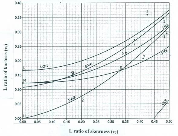
Figure 1 Diagram of L moment quotients, showing PDF of two and three fitting parameters (^{Hosking & Wallis, 1997}). 

Fitting source PDF

Exclusively, the LP3 distribution was applied with the moments method in the logarithmic dominion (^{WRC, 1977}; ^{Campos-Aranda, 2015}); while ^{Botto et al. (2017)} fit it as a PT3 based on the logarithmic L quotients. The rest of the distributions from Table 1 were fit with the method of L moments, following the procedures described by ^{Hosking and Wallis (1997)}. In all cases the standard error of fit (SEF) was evaluated.

Standard error of fit

The standard error of fit is the most common indicator for contrasting PDF against real data (^{Chai & Draxler, 2014}). It was established in the mid-1970s (^{Kite, 1977}), and has been applied in Mexico using the empirical formula of Weibull (^{Benson, 1962}). Now, its application is recommended for use with the formula of Cunnane (Equation (18)), according to ^{Stedinger (2017)}, leading to non-exceedance probabilities (p) approximately unbiased for many PDF; that is:

The expression for the standard error of fit is:

In which Q_i are annual maximum flows ordered from least to highest and whose number is n, and Q^i are the estimated maximum flows for the probability estimated with Equation (18) and the PDF that contrasts. np is the number of fitting parameters of the PDF, with three for the five to be applied.

Flood registers to be analyzed

To develop the numerical applications, we chose to process the seven largest registers (43 ≤ n ≤ 56) of hydrometric information processed by ^{Campos-Aranda (2014)} of Hydrological Region Num. 10 (Sinaloa), Mexico, corresponding to the Huites, Santa Cruz, Jaina, Naranjo, Acatitán, Zopilote and El Bledal stations. Table 2 cites two general characteristics and the L moment ratio values of the seven selected stations.

Figure 1 shows the graphic position of each register, according to its asymmetry and kurtosis L quotient. We deduced that the convenient PDF (because of their closeness) are the following: in Huites PAG, in Santa Cruz LOG, in Jaina GEV, in Naranjo PT3, in Acatitán LN3, in Zopilote PAG and in El Bledal GVE.

Verification of register randomness

For the results of the FFA to be exact, the register of annual maximum flows to be processed must have been generated by a stationary random process, which implies that it has not changed over time. Therefore, the flood register should integrate independent data, exempt of deterministic components.

To test this, we applied the Wald-Wolfowitz Test, which is a non-parametric test used by ^{Bobée and Ashkar (1991)}, ^{Rao and Hamed (2000)}, and ^{Meylan, Favre, and Musy (2012)} to verify independence and stationarity in registers of annual maximum flows. Its application in the seven selected registers showed that they are integrated by independent random data.

The best PDF, according to minimum DA

Based on L moment ratios from Table 2, we used Equation (17) to find the two minimum DA and, in this way, define the two most suitable PDF in Table 3. The second option will be used in the Huites and Zopilote stations since ^{Botto et al. (2017)} did not establish the Generalized Pareto as the parent distribution in Table 1.

Design predictions and their correction

Table 4 presents the estimated predictions with each of the most convenient PDF for the five return periods that ^{Botto et al. (2017)} analyzed. Moreover, their correction factors (y^) calculated with Equation (3) are shown, and finally, we have the corrected DF (Q^Tr*) due to hydrological uncertainty.

We can observe in Table 4 that the smallest corrections (y^) in the Tr = 50 years were less than 1% in the Santa Cruz, Jaina and El Bledal stations, and the largest was 5.6% in Naranjo. In the Tr = 1000 years, the smallest correction is 14.9% in Santa Cruz and the largest rises to 43.9% in Naranjo. In general, the corrections of the LP3 distribution are the largest, while the smallest are those of the LOG model. This is most likely related to the density of the right tail (^{El Adlouni, Bobée, & Ouarda, 2008}) of these two PDFs under precept application in the USA and England.

REFERENCES

Benson, M. A. (1962). Plotting positions and economics of engineering planning. Journal of Hydraulics Division, 88(6), 57-71. [ Links ]
Bobée, B. & Ashkar, F. (1991). The Gamma Family and derived distributions applied in Hydrology. Chapter 1: Data requirements for hydrologic frequency analysis (pp. 1-12). Littleton, USA: Water Resources Publications. [ Links ]
Botto, A., Ganora, D., Laio, F., & Claps, P. (2014). Uncertainty compliant design flood estimation. Water Resources Research, 50(5), 4242-4253. [ Links ]
Botto, A., Ganora, D., Claps, P., & Laio, F. (2017). Technical note: Design flood under hydrological uncertainty. Hydrology and Earth System Sciences, 21(7), 3353-3358. [ Links ]
Burn, D. H. (2003). The use of resampling for estimating confidence intervals for single site and pooled frequency analysis. Hydrological Sciences Journal, 48(1), 25-38. [ Links ]
Campos-Aranda, D. F. (2014). Análisis regional de frecuencia de crecientes en la Región Hidrológica No. 10 (Sinaloa), México. 2: contraste de predicciones locales y regionales. Agrociencia, 48(3), 255-270. [ Links ]
Campos-Aranda, D. F. (2015). Introducción a la hidrología urbana. En: Técnicas estadísticas y probabilísticas (pp. 25-51). San Luis Potosí, México: Edición del autor (ISBN-970-95118-1-5). 307 páginas. [ Links ]
Chai, T., & Draxler, R. R. (2014). Root mean square error (RMSE) or mean absolute error (MAE)? - Arguments against avoiding RMSE in the literature. Geoscientific Model Development, 7, 1247-1250. [ Links ]
Cheng, K. S., Chang, J. L., & Hsu, C. W. (2007). Simulation of probability distributions commonly used in hydrological frequency analysis. Hydrological Processes, 21(1), 51-60. [ Links ]
El Adlouni, S., Bobée, B., & Ouarda, T. B. M. J. (2008). On the tails of extreme event distributions in hydrology. Journal of Hydrology, 355(1-4), 16-33. [ Links ]
Greenwood, J. A., Landwehr, J. M., Matalas, N. C., & Wallis, J. R. (1979). Probability weighted moments: Definition and relation to parameters of several distributions expressible in inverse form. Water Resources Research, 15(5), 1049-1054. [ Links ]
Hosking, J. R., & Wallis, J. R. (1997). Regional frequency analysis. An approach based on L-moments. Chapter 2: L-moments and Appendix: L-moments for some specific distributions. (pp. 14-43, 191-209). Cambridge, UK: Cambridge University Press. [ Links ]
Kite, G. W. (1977). Frequency and risk analyses in hydrology. Chapter 3: Frequency distributions. General and chapter 12: Comparison of frequency distributions (pp. 27-39, 156-168). Fort Collins, USA: Water Resources Publications. [ Links ]
Kjeldsen, T. R., Lamb, R., & Blazkova, S. D. (2014). Uncertainty in flood frequency analysis. In: Beven, K., & Hall, J. (eds.). Applied Uncertainty analysis for flood risk management (pp. 153-197). London, UK: Imperial College Press. [ Links ]
Merz, R., & Blöschl, G. (2008). Flood frequency hydrology: 1. Temporal, spatial and causal expansion of information. Water Resources Research, 44(8), 1-17. [ Links ]
Meylan, P., Favre, A. C., & Musy, A. (2012). Predictive Hydrology. A frequency analysis approach. Chapter 3: Selecting and checking data series. (pp. 29-70). Boca Raton, USA: CRC Press. [ Links ]
Rao, A. R., & Hamed, K. H. (2000). Flood frequency analysis. Theme 1.8: Tests on hydrologic data (pp. 12-21) and Chapter 3: Probability Weighted Moments and L-Moments. (pp. 53-72). Boca Raton, USA: CRC Press . [ Links ]
Stedinger, J. R. (2017). Flood frequency analysis. Chapter 76 (pp. 76.1-76.8). In: Singh, V. P. (ed.). Handbook of applied hydrology. New York, USA: McGraw-Hill Education. [ Links ]
Stedinger, J. R., Vogel, R. M., & Foufoula-Georgiou, E. (1993). Frequency analysis of extreme events. In: Maidment, D. R. (ed.). Handbook of Hydrology (pp. 18.1-18.66). New York, USA: McGraw-Hill, Inc. [ Links ]
WRC, Water Resources Council. (1977). Guidelines for determining flood flow frequency. Bulletin #17A of the Hydrology Committee. Washington, DC, USA: Water Resources Council. [ Links ]
Yue, S., & Hashino, M. (2007). Probability distribution of annual, seasonal and monthly precipitation in Japan. Hydrological Sciences Journal, 52(5), 863-877. [ Links ]
Received: February 04, 2020; Accepted: April 08, 2020
Este es un artículo publicado en acceso abierto bajo una licencia
Creative Commons