


 nueva página del texto (beta)
 Inglés (pdf)
 Artículo en XML
 Referencias del artículo
 Enviar artículo por email
 Citado por SciELO
  Similares en
SciELO
Similares en
SciELO 
 Permalink
Introduction
The composition and dynamics of terrestrial small-mammal communities in the Neotropics are to date poorly documented (Mares 1982; Lacher and Mares 1986; Mares and Ernest 1995; Willig et al. 2000; Owen 2013). Accordingly, studies of terrestrial small-mammal communities are increasingly the focus of intensive studies. However, the majority of these studies are either broad-scale comparisons of faunal communities (Ojeda et al. 2000; Willig et al. 2000), or are evaluations of a community situated well within the geographic and ecologic boundaries of the ecoregion being evaluated (e. g., Ribeiro and Marinho-Filho 2005; Bernardes 2006; Becker et al. 2007; Magnusson et al. 2010). With the increasing fragmentation of ecoregions, it will be increasingly important to assess community composition and dynamics in marginal patches of a particular ecoregion (Santos 2008; Owen 2013). Faunal members of such communities are presumed to be living near the limits of their capabilities in terms of their abiotic (e. g., soils, weather, climate) and biotic environment (vegetation composition and structure, predators, competitors). Moreover, such communities are likely to be sensitive to extrinsic variables such as climate change and anthropogenic changes in land use (Willig et al. 2000; Carnaval and Moritz 2008; Meserve et al. 2011; Owen 2013; de la Sancha et al. 2014). Importantly, a detailed understanding of the responses of rodent communities and their more common species to both biotic and abiotic variations in their environment is necessary for developing predictive models for the emergence of rodent-borne zoonotic pathogens (Glass et al. 2002; Goodin et al. 2006; Keesing et al. 2010; Han et al. 2015; Eastwood et al. 2018; Morand et al. 2019).
Most of eastern Paraguay is within the historical distribution of the Upper Paraná Atlantic Forest (UPAF), which is a Biodiversity Hotspot and Conservation Priority Area (Myers et al. 2000; Willig et al. 2000). This ecoregion has experienced extensive land-use conversion for ranching and agriculture resulting in less than 7 % of the original footprint remaining (Klink and Moreira 2002; Klink and Machado 2005; Silva et al. 2006; Huang et al. 2007, 2009). This study evaluates the temporal dynamics and particularly the effects of the El Niño / Southern Oscillation (ENSO) and precipitation on the sigmodontine rodent communities occupying three types of habitat degradation, near the western limit of the UPAF in eastern Paraguay. We hypothesized that substantial fluctuations in rodent species diversity and sigmodontine population abundance would result from fluctuations in the abiotic variables mentioned above, and that these effects would be dissimilar in the three communities sampled, due to differing levels of habitat degradation. Moreover, we expected that some species would be more responsive to climatic (abiotic) fluctuations, whereas others might be more sensitive to habitat degradation.
Materials and Methods
Study Site. The study was conducted in the Reserva Natural del Bosque Mbaracayú (RNBM), a natural reserve of ca. 65,000 ha in Canindeyú Department, northeastern Paraguay (Figure 1). This site is located within climate type Cfa (temperate, without dry season, hot summer—Peel et al. 2007). The RNBM is located near the western margin of the Upper Paraná Atlantic Forest (UPAF—depicted as Moist Broadleaf Forest in the biome map of Olson et al. 2001), and receives an annual average precipitation of approximately 1550 mm (https://crudata.uea.ac.uk/cru/data/hrg/cru_ts_4.02/ge/, accessed 17 March 2019).
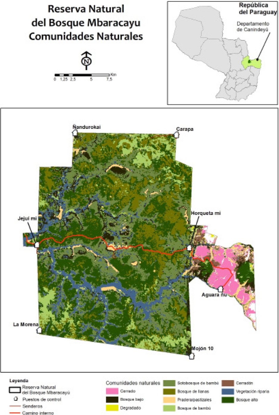
Figure 1 Map of the Reserva Natural del Bosque Mbaracayú and its location within Paraguay, and land cover based on supervised classification of satellite imagery combined with extensive ground-truthing using habitat categorization by local Ache (Indigenous) people. See text for location and description of sampling grids. Map based on Naidoo and Hill (2006) and Peña-Chocarro et al. (2010).
The three sampling grids were evaluated based on an extensive series of vegetation structural characteristics, measured at each of the trap stations in each grid. Means of these vegetation measures were used as general measures for each grid. These were standardized to a mean of zero and standard deviation of one, to mitigate against effects of character size. Eigenvectors were extracted from the correlation matrix of standardized characters and evaluated using Principal Component Analysis (PCA; Sneath and Sokal 1973). Following preliminary analyses, six characters were included in the final PCA, as being important descriptors of both forest quality and rodent habitat: dead wood on ground, maximum canopy height, distance to nearest trees, percentage coverage by forbs, logs (fallen trees) in vicinity, and presence of orange trees. Degradation levels were judged to be positively associated with the first two principal components, which together represented 95% of the variance (Table 1). Thus, more degraded (poorer) forest habitat is associated with forbs, logs (fallen trees), and orange trees (Citrus aurantium, an introduced species which has acclimatized in disturbed forest). Less degraded forest habitat is associated with more dead wood (fallen branches, not fallen trees), higher canopy and lower distance to the nearest tree. Based on these criteria, Grid B (centered at -24.141o S, -55.366o W) was designated as “least degraded”, Grid A (-24.123o S, -55.505o W) was “moderately degraded”, and Grid G (-24.131o S, -55.537o W) was “most degraded”. Grid names and designations are consistent with other publications based on data developed in this project.
Table 1 Loadings of six vegetation measures on principal components 1 and 2, and percent of variance explained by these two components.
| Vegetation | PC-1 | PC-2 |
|---|---|---|
| Percent coverage by forbs | 0.972 | 0.185 |
| Percent coverage by deadwood | -0.788 | 0.602 |
| Maximum canopy height | -0.816 | -0.533 |
| Minimum distance to trees | 0.245 | -0.942 |
| Presence of fallen trees | 0.947 | -0.140 |
| Presence of orange trees | 0.960 | 0.233 |
| % of variance | 62.2 | 32.8 |
Sampling methods and protocol. Each 12 by 12 sampling grid consisted of 144 trap stations, with the traps placed 10 m apart. Sampling was conducted six times (July and November 2015, February, July and November 2016, and February 2017). July is winter, and typically dry, whereas November is the beginning of the summer and the peak of the rainy season, and February is the end of summer, with intermediate rainfall levels. In each sampling session, traps were opened for five nights on each grid. In the first sampling session two traps were placed at each station (one trap on the ground, one on a plywood platform 2 to 3 meters above the ground, in vines or branches). Thereafter (for the remaining five sampling sessions) three traps were placed at each station (two on the ground, one on a platform above ground). Thus, 432 traps were open each night for the remaining five sampling sessions resulting in 2,160 trap-nights per sampling session with the total effort for the six sampling sessions of the study being 36,720 trap-nights.
Environmental data. Monthly multivariate ENSO index (MEI) values (Wolter and Timlin 1993, 1998) were downloaded from the Physical Sciences Division of the Earth Sciences Laboratory, U.S. National Oceanic and Atmospheric Administration (https://www.esrl.noaa.gov/psd/enso/mei/data/meiv2.data) for the time period beginning one year before rodent sampling began, until the final sampling period. Precipitation data (Precip) were obtained for the same time period from the Climatic Research Unit of the University of East Anglia accessed via a Google Earth application ((https://crudata.uea.ac.uk/cru/data/hrg/cru_ts_4.02/ge/). Precipitation data are presented as 0.5-degree grid averages. Because the RNBM lies approximately equally on two of the grid squares, the precipitation values for those two squares were averaged to calculate monthly precipitation values for the study site. Monthly precipitation values were also downloaded for the 30 years prior to the study (1984 to 2013) to calculate historical monthly precipitation means and standard deviations. Monthly precipitation anomaly values (Anom) were calculated by subtracting the monthly means from the recorded precipitation amounts during the study. To evaluate the effect of ENSO on precipitation at the study site, Pearson product-moment correlations were calculated between MEI and Precip (current month and monthly lagged values for from 1-6 months), and between MEI and Anom (current and lagged for from 1 to 6 months).
Correlations between rodent community measures and abiotic measures. For comparison with rodent community and population measures, MEI, precipitation and precipitation anomaly values were listed for each of the six sampling months, as well as cumulative MEI, precipitation and anomaly for the two, three, four, six, and twelve-month periods ending with each sampling month (MEI1 - MEI12, Precip1 - Precip12, Anom1 - Anom12). Total sigmodontine abundance (all species included) and species diversity (Shannon index) were calculated for each of the three grids and each of the six sampling sessions. Because abundance values may be expected to conform to a Poisson distribution, a Shapiro-Wilk test was conducted, which failed to reject the null hypothesis of normality (W = 0.96, P = 0.602). Thus, we did not transform the abundance values. Product-moment correlations were then calculated between each of these two rodent community measures and each of the climatic variables. We arbitrarily considered correlations with an absolute value > 0.70 to indicate potential climatic predictors (MEI, precipitation and precipitation anomaly) of fluctuations in population measures (species diversity, total abundance and species abundances,), which corresponds to a 93 % confidence interval around r = 0. All calculations were made in Microsoft Excel™, with the exception of calculations pertaining to the principal components analyses, which were conducted using NTSYSpc ver. 2.2 (Rohlf 2005).
Results
Based on monthly precipitation data from the 30 years prior to this study (1984 to 2013), October - December (spring and early summer) is normally the peak rainy season at the study site, with another shorter period in April - May (autumn). The second period is much less consistent, having a higher standard deviation of precipitation amount than any other month of the year.
Among the abiotic variables, the multivariate ENSO index (MEI) correlated weakly with the current month for both precipitation and precipitation anomaly, with the correlation coefficients for both decreasing non-monotonically for increasing lag times, with very little association after three months. For current and all lagged periods, MEI correlated with the precipitation anomaly than with precipitation, indicating that greater than normal rainfall is received during periods of higher MEI values (El Niño events). However, no value of r was greater than 0.29, and MEI, anomaly and precipitation were treated as independent abiotic variables, for the comparisons with species diversity and sigmodontine and species abundances.
A total of 1,632 captures (4.4 % overall trap success) was recorded in the sampling, involving 1,021 individual animals (611 recaptures). Overall, 13 species were encountered, two of which remain unidentified. Sigmodontine species richness varied from 4 to 6 on Grid B (least degraded), 4 to 7 on Grid A (moderately degraded), and 4 to 7 on Grid G (most degraded). Akodon montensis was by far the commonest species, with 64.6 % of the individuals, followed by Hylaeamys megacephalus (17.3 %) and Oligoryzomys nigripes (9.0 %, Table 2). Shannon species diversity varied from 0.70 to 1.11 on Grid B, 0.73 to 1.32 (Grid A), and 1.00 to 1.41 (Grid G). Total sigmodontine abundance (species combined) ranged from 17 to 88 (B), 27 to 111 (A), and 23 to 53 (G; Table 3).
Table 2 Summary of species encountered on each grid, for all six sampling sessions combined. Least, moderate and most refer to level of habitat degradation, as evaluated using a principal components analysis of six environmental variables, measured at each of 144 trap stations on each grid, and averaged for the grid.
| Grid B (least) | Grid A (moderate) | Grid G (most) | Overall | |||||
| Species | # indiv. | Percent. | # indiv. | Percent. | # indiv. | Percent. | # indiv. | Percent. |
| Akodon montensis | 254 | 71.9% | 279 | 64.7% | 127 | 53.6% | 660 | 64.6% |
| Calomys callosus | 1 | 0.3% | 2 | 0.5% | 8 | 3.4% | 11 | 1.1% |
| Euroryzomys russatus | 2 | 0.6% | 0 | 0.0% | 0 | 0.0% | 2 | 0.2% |
| Hylaeamys megacephalus | 45 | 12.7% | 75 | 17.4% | 57 | 24.0% | 177 | 17.3% |
| Juliomys pictipes | 2 | 0.6% | 0 | 0.0% | 0 | 0.0% | 2 | 0.2% |
| Necromys lasiurus | 0 | 0.0% | 3 | 0.7% | 0 | 0.0% | 3 | 0.3% |
| Oecomys mamorae | 0 | 0.0% | 1 | 0.2% | 0 | 0.0% | 1 | 0.1% |
| Oligoryzomys mattogrossae | 9 | 2.5% | 17 | 3.9% | 10 | 4.2% | 36 | 3.5% |
| Oligoryzomys nigripes | 31 | 8.8% | 40 | 9.3% | 21 | 8.9% | 92 | 9.0% |
| Oligoryzomys sp. | 5 | 1.4% | 12 | 2.8% | 6 | 2.5% | 23 | 2.3% |
| Rhipidomys macrurus | 1 | 0.3% | 0 | 0.0% | 2 | 0.8% | 3 | 0.3% |
| Sooretamys angouya | 2 | 0.6% | 2 | 0.5% | 5 | 2.1% | 9 | 0.9% |
| Oryzomyine sp. | 1 | 0.3% | 0 | 0.0% | 1 | 0.4% | 2 | 0.2% |
| Totals | 353 | 100.0% | 431 | 100.0% | 237 | 100.0% | 1021 | 100.0% |
Table 3 Species richness and Shannon diversity and total abundance for sigmodontine rodents on three sampling grids during six sampling sessions in the Reserva Natural del Bosque Mbaracayú. Grid B had the least degraded habitat, Grid A was moderately degraded, and Grid G the most degraded. See text for further description of grid habitats.
| Year | Month | Session | RICH-B | RICH-A | RICH-G | DIV-B | DIV-A | DIV-G | ABUN-B | ABUN-A | ABUN-G |
| 2015 | Jul | 2 | 4 | 7 | 6 | 0.94 | 1.01 | 1.22 | 82 | 111 | 53 |
| 2015 | Nov | 3 | 5 | 6 | 4 | 0.70 | 0.73 | 1.00 | 71 | 79 | 47 |
| 2016 | Feb | 4 | 5 | 6 | 7 | 0.97 | 1.32 | 1.30 | 88 | 63 | 52 |
| 2016 | Jul | 5 | 6 | 5 | 6 | 1.11 | 1.18 | 1.41 | 40 | 50 | 32 |
| 2016 | Nov | 6 | 5 | 4 | 5 | 1.00 | 0.87 | 1.31 | 17 | 27 | 23 |
| 2017 | Feb | 7 | 6 | 6 | 5 | 0.89 | 1.20 | 1.28 | 55 | 101 | 30 |
Correlations between climatic and population measures were quite variable. In general, species diversity was negatively correlated with the three sets of climatic variables (MEI, precipitation, precipitation anomaly, and their cumulative values; Figure 2). In contrast, total sigmodontine abundance was positively correlated with the three climatic variables.
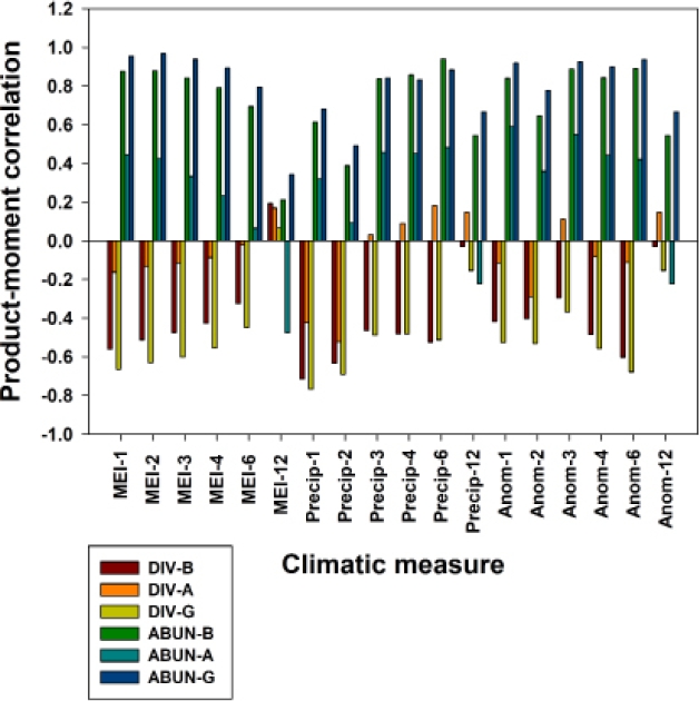
Figure 2 Correlograms showing product-moment correlations between sigmodontine species diversity and total abundance with MEI, precipitation and precipitation anomaly, shown for 1, 2, 3, 4, 6 and 12-month cumulative values. Grid B, least degraded; Grid A, moderately degraded; Grid G, most degraded.
Predictors of species diversity. Notwithstanding a generally negative correlation with the climatic variables, species diversity appeared to be only loosely associated with those variables which we evaluated (Table 4), with only Grids B and G (least and most degraded) showing an “important” (absolute value > 0.70) correlation with current month precipitation, and no other climatic variable. On both grids, species diversity correlated most strongly with current-month values of MEI and precipitation, generally deceasing with increasing cumulative values. In contrast, species diversity on these same two grids correlated best with the six-month cumulative value for precipitation anomaly (Figure 2). On the moderately degraded grid (A), species diversity was negatively correlated with nearly all climatic variables, although strongly with none (Table 4), and the strongest correlations were with the two-month cumulative values of precipitation and precipitation anomaly (Figure 2).
Table 4 Climatic variables arranged in order from highest to lowest correlation coefficient with each community measure (sigmodontine species diversity (Shannon Index) and total sigmodontine abundance), for each grid (B, least degraded; A, moderately degraded; G, most degraded). Climatic measures with negative correlation coefficients are shown in parentheses. Measures with absolute value of correlation coefficient > 0.70 are shown in bold face.
| Species diversity | Total abundance | ||||
|---|---|---|---|---|---|
| Grid B | Grid A | Grid G | Grid B | Grid A | Grid G |
| MEI-12 | Precip-6 | MEI-12 | Precip-6 | Anom-1 | MEI-2 |
| (Anom-12) | MEI-12 | (Anom-12) | Anom-6 | Anom-3 | MEI-1 |
| (Precip-12) | Anom-12 | (Precip-12) | Anom-3 | Precip-6 | MEI-3 |
| (Anom-3) | Precip-12 | (Anom-3) | MEI-2 | Precip-3 | Anom-6 |
| (MEI-6) | Anom-3 | (MEI-6) | MEI-1 | Precip-4 | Anom-3 |
| (Anom-2) | Precip-4 | (Precip-4) | Precip-4 | MEI-1 | Anom-1 |
| (Anom-1) | Precip-3 | (Precip-3) | Anom-4 | Anom-4 | Anom-4 |
| (MEI-4) | (MEI-6) | (Precip-6) | MEI-3 | MEI-2 | MEI-4 |
| (Precip-3) | (Anom-4) | (Anom-1) | Anom-1 | Anom-6 | Precip-6 |
| (MEI-3) | (MEI-4) | (Anom-2) | Precip-3 | Anom-2 | Precip-3 |
| (Precip-4) | (Anom-6) | (MEI-4) | MEI-4 | MEI-3 | Precip-4 |
| (Anom-4) | (Anom-1) | (Anom-4) | MEI-6 | Precip-1 | MEI-6 |
| (MEI-2) | (MEI-3) | (MEI-3) | Anom-2 | MEI-4 | Anom-2 |
| (Precip-6) | (MEI-2) | (MEI-2) | Precip-1 | Precip-2 | Precip-1 |
| (MEI-1) | (MEI-1) | (MEI-1) | Precip-12 | MEI-6 | Precip-12 |
| (Anom-6) | (Anom-2) | (Anom-6) | Anom-12 | (Precip-12) | Anom-12 |
| (Precip-2) | (Precip-1) | (Precip-2) | Precip-2 | (Anom-12) | Precip-2 |
| (Precip-1) | (Precip-2) | (Precip-1) | MEI-12 | (MEI-12) | MEI-12 |
Predictors of sigmodontine abundance. Sigmodontine abundance was strongly positively correlated with 11 of the 18 climatic variables on Grid B (least degraded), showing an immediate increase with higher MEI and anomaly values, as well as with three, four and six-month cumulative precipitation. No strong correlations were found between abundance and twelve-month cumulative values (Table 4). Similarly, abundance on Grid G (most degraded) showed strong correlations with 13 of the 18 climatic variables, and no strong correlations with twelve-month cumulative values. In contrast, Grid A (moderately degraded) exhibited no strong correlation of sigmodontine abundance with any climatic variable.
Abundant species, species diversity and total abundance. The three most abundant species in this study were Akodon montensis, Hylaeamys megacephalus and Oligoryzomys nigripes, with 64.6 %, 17.3 % and 9.0 % of all individuals, respectively (Table 2). Because A. montensis represents nearly two-thirds of the overall population, abundance levels of this species generally correlate strongly and positively with total sigmodontine abundance (Figure 3). Moreover, an increased proportion of A. montensis corresponds on each grid with a decrease in species diversity, as measured by the Shannon Index (Figure 4).
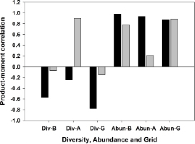
Figure 3 Correlogram showing product-moment correlations between Akodon montensis and Hylaeamys megacephalus population abundances, with species diversity and total sigmodontine abundance on three sampling grids. Grid B, least degraded; Grid A, moderately degraded; Grid G, most degraded. Black bars, Akodon montensis; gray bars, Hylaeamys megacephalus.
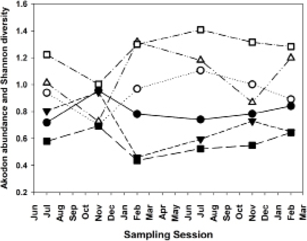
Figure 4 Akodon montensis population abundances (expressed as percentage of total sigmodontine abundance) and Shannon species diversity. Closed figures, A. montensis abundances; open figures, Shannon diversity. Circles, Grid B; triangles, Grid A; squares, Grid G.
The three most abundant species exhibited differing correlation patterns with total sigmodontine abundance, in the different levels of habitat degradation. Akodon montensis was consistently strongly correlated with total abundance, across the three grids. In contrast, H. megacephalus was strongly correlated with total abundance on Grids B and G (least and most degraded), and essentially uncorrelated on Grid A (moderately degraded), and O. nigripes most strongly correlated on Grids B and A, and uncorrelated on Grid G (most degraded; Figure 5).
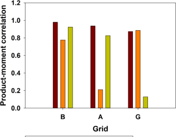
Figure 5 Correlations of population abundances of Akodon montensis (brown bar), Hylaeamys megacephalus (orange bar), Oligoryzomys nigripes (lemon bar), with abundances of all sigmodontine species combined.
As mentioned, on Grid A (moderately degraded), H. megacephalus showed only a low correlation with total abundance, although it showed a strong positive correlation with species diversity. On grids A and G, A. montensis and H. megacephalus showed strongly contrasting responses in the sampling session of February 2016 (the end of the strong El Niño event of late 2015), with Akodon decreasing and Hylaeamys increasing, after which percentages returned to earlier levels. In contrast, neither of these two species were affected by the El Niño event on Grid B (least degraded; Figure 6).
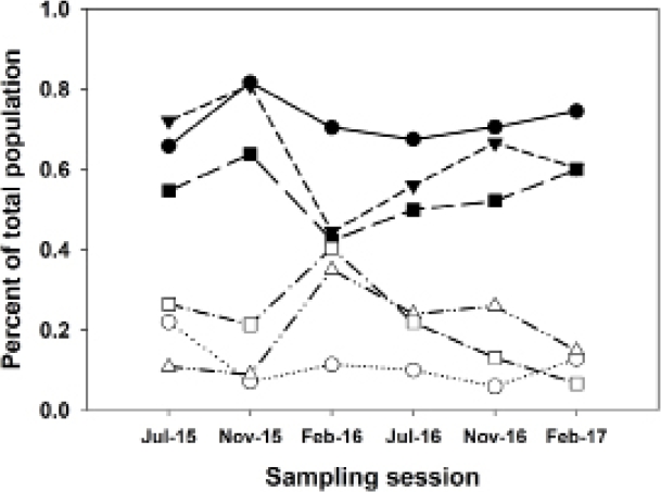
Figure 6 Chart showing relationships of population abundances of Akodon montensis and Hylaeamys megacephalus, shown as percentages of total sigmodontine abundance for each sampling session on each grid. Solid symbols, Akodon montensis; open symbols, Hylaeamys megacephalus. Circles, Grid B (least degraded); triangles, Grid A (moderately degraded); squares, Grid G (most degraded). Note the strongly contrasting changes in A. montensis and H. megacephalus in February 2016, at the end of the strong El Niño event, on Grids A and G. However, the populations on Grid B (least degraded) were not affected by the El Niño event.
Discussion
The Sigmodontine community composition and relative abundances of the three most abundant species in this study were similar to those from other studies in the Atlantic Forest habitat of the RNBM (Owen et al. 2010; Eastwood et al. 2018). However, there are considerable differences between this community and others in Atlantic Forest (e. g., Cademartori et al. 2004; Carmignotto and Aires 2011; Melo et al. 2011; Galiano et al. 2013; Maestri and Marinho 2014; Barros et al. 2015; Machado et al. 2019). One noteworthy difference was that while Hylaeamys megacephalus was abundant on all sites in our study, it is absent in more southerly latitudes, reflecting its tropical distribution from the north coast of Venezuela southward across Amazonia and terminating in east-central Paraguay. Akodon montensis reaches the western limit of its more subtropical distribution in eastern Paraguay and northern Argentina, as does Oligoryzomys nigripes, which is distributed from northeastern Brazil southward to Uruguay (D’Elía and Pardiñas 2015). Thus, although each is widely distributed, the three most abundant species in this study are all near the limits of their distributions.
Higher overall sigmodontine abundance was generally associated with lower species diversity in this study, indicating that the diversity index was driven primarily by evenness, rather than species richness. In fact, species richness varied little throughout the study, whereas abundances varied substantially. This finding contrasts with those reported in other studies in which species diversity and abundance were both highest in the same habitat or in the same season (e. g., Gastal 1997; Alho 2005; Asfora et al. 2009).
Hannibal and Neves-Godoi (2015) found Hylaeamys megacephalus to be more abundant and more broadly distributed among habitats than Akodon montensis in a study in Mato Grosso do Sul, Brazil. Similarly, Santos (2008) found H. megacephalus to be more abundant than an unidentified Akodon species in an Amazon-Cerrado interface area. In our study, increased overall abundance was due primarily to increased abundance of Akodon montensis. However, on Grids A and G (moderately and most degraded) in one sampling session (February 2016) an increase in overall abundance resulted from an increase in Hylaeamys megacephalus, while the proportion of A. montensis in the population decreased. This sampling session coincided with the end of an “exceptionally intense” El Niño event (Dirección Nacional de Aeronáutica Civil 2016). This inverse relationship between the two most abundant species, apparently in response to the El Niño event, was negligible on Grid B (least degraded). To our knowledge, this complex interaction of population response by these two abundant species has not been reported elsewhere, and certainly bears further study and confirmation.
Effects of habitat degradation. Several important studies have documented differences in sigmodontine species diversity and abundance in response to different habitat quality or degradation (e. g., Gastal 1997; Cerqueira et al. 2003; Alho 2005; Melo et al. 2011; Sponchiado et al. 2012; Galiano et al. 2013; de la Sancha et al. 2014). Results of the present study also document such differences associated with differing levels of habitat degradation.
Habitat degradation affects species diversity. Species diversity increased with increased habitat degradation. Diversity was highest in the most degraded habitat (Grid G; Shannon Index H = 1.25 ± 0.135 across six sampling sessions), lowest in the least degraded habitat (Grid B, H = 0.94 ± 0.135), and intermediate in the moderately degraded habitat (Grid A, H = 1.05 ± 0.223). However, the effect of habitat degradation was less consistent in the moderately degraded habitat, as indicated by the higher standard deviation of species diversity levels across sampling sessions.
Habitat degradation affects overall sigmodontine abundance. The moderately degraded habitat had the highest sigmodontine abundance. Abundance was not associated monotonically with degradation extent. Grid A (moderately degraded) had the highest average abundance ( 72 ± 31.6), as well as being the least consistent (highest standard deviation). The most degraded habitat (Grid G) consistently had the lowest abundance ( 40 ± 12.8), and the least degraded habitat (Grid B) was intermediate in both mean and standard deviation ( 59 ± 27.0).
Habitat degradation affects different species differently. Of the three most abundant species, Akodon montensis abundance generally correlated highly with overall sigmodontine abundance on all three grids. Nevertheless, it showed a strong reduction in relative abundance (percentage of overall population) on Grids B and G in the February 2016 sample, at the end of a strong El Niño event. Hylaeamys megacephalus generally correlated strongly with overall abundance on Grids B and G (least and most degraded), but not on Grid A (moderately degraded). However, on both Grids G and A, H. megacephalus strongly increased in relative abundance in the February 2016 sample, benefitting apparently from either the reduction in A. montensis, or the heavy rains of the preceding several months, or both. Oligoryzomys nigripes abundance correlated with overall abundance on B and A (least and moderately degraded), but did not coincide with the overall abundance variations on Grid G (most degraded), apparently not benefiting from conditions that produced increases in the other two species.
Effects of climatic fluctuations. Numerous studies have also demonstrated effects of climatic variability (particularly precipitation) on sigmodontine community diversity, abundance and composition (e. g., D’Andrea et al. 1999; Melo et al. 2011; Lacher 2012; Sponchiado et al. 2012; Galiano et al. 2013). The present study supports the importance of climatic variability for sigmodontine community parameters, as well as for abundances of common species.
Climate variability affects species diversity. The Multivariate ENSO Index (MEI) of the current month was moderately negatively correlated with species diversity on Grids B and G (least and most degraded) with decreasing strength of correlation with increasing cumulative lengths of MEI scores. On Grid A (moderately degraded), MEI showed only very weak correlations with diversity. Current-month precipitation was also negatively correlated with species diversity on Grids B and G, with two-month cumulative precipitation slightly less strongly correlated. On Grid A, the two-month cumulative precipitation showed the strongest correlation with diversity, and present-month precipitation at a slightly lower correlation strength. In contrast to MEI and precipitation, species diversity was most strong correlated (negatively) with four- and six-month cumulative anomaly values on Grids B and G. Again, Grid A did not follow the response pattern of the other grids, showing only low correlation values with precipitation anomaly.
Climate variability affects overall sigmodontine abundance. MEI was strongly positively correlated with overall sigmodontine abundance for Grids B and G, for current month and cumulative MEI values of up to six months, decreasing to low correlation values at 12 months. Overall abundance on Grid A was much less strongly correlated (also positively) with MEI current and cumulative values. Precipitation correlated most strongly with sigmodontine abundance on Grids B and G in the three-, four- and six-month accumulations, again with Grid A less strongly correlated. Precipitation anomaly reflected this same pattern, as well as strong correlations with current-month anomaly for Grids B and G, with Grid A again less strongly correlated.
Climate variability affects common species differently. On Grid B (least degraded), Akodon montensis and Hylaeamys megacephalus population percentages varied very little across the six sampling sessions. Although the overall populations varied considerably, the percentages of these two species remained relatively constant. On Grids A and G, pronounced variation was seen, with Akodon increasing and Hylaeamys decreasing in the first part of the El Niño event of late 2015 (Dirección Nacional de Aeronáutica Civil 2016), and then reversing those trends toward the end of that event, with Akodon and Hylaeamys of nearly equal proportions in February 2016, after which both populations returned to pre-El Niño percentages, and Hylaeamys decreasing nearly to zero on Grid G (most degraded) by February 2017.
In this two-year study, substantial fluctuations in rodent species diversity and sigmodontine population abundance were noted, and these were often correlated with fluctuations in the abiotic variables examined. We also found that these effects were dissimilar in the three habitats sampled, representing differing levels of habitat degradation. However, this dissimilarity was expressed as an unexpected pattern. In fact, a particularly interesting result of this investigation was that species diversity and overall sigmodontine abundance were both only poorly correlated with abiotic variables on the moderately degraded habitat (Grid A), and also were more highly variable on that grid, than in the least and most-degraded habitats. As a result, populations on the least- and most-degraded grids could be substantially predicted by the abiotic variables, whereas populations on the moderately degraded grid were highly variable, and apparently responding to biotic or abiotic factors which were not included in our study.
Another noteworthy result was that, although several community and species population measures which were correlated with climatic variables, none showed important correlations with 12-month cumulative values of these variables. In other words, the community and its populations were not responsive to cumulative precipitation of the entire preceding year, but were responsive to the preceding half-year’s events. We did not test for cumulative values between 6 and 12 months, and further investigation is needed to determine the duration of cumulative climatic events which are important to the sigmodontine populations. Additionally, the deviation of the community and population responses in the moderately habitat (Grid A) require better understanding, and may be particularly important in the context of complex interactions of populations of common species such as Akodon montensis and Oligoryzomys nigripes, which hosts to Jabora and Juquitiba hantaviruses, respectively (Eastwood et al. 2018).
Finally, we found that some species were more responsive to climatic (abiotic) fluctuations, whereas others were more sensitive to habitat degradation. Akodon montensis closely followed overall abundance (which correlated positively with climatic variation) on all three grids, whereas Hylaeamys megacephalus did so only in the least- and most-degraded habitats, and Oligoryzomys nigripes only in the least- and moderately-degraded habitats.
Akodon montensis is primarily terrestrial, although it may also ascend lianas or low branches of bushes (Machado et al. 2019). It is primarily an Atlantic Forest species, also occurring in gallery forest of the Cerrado, whose distribution extends from Minas Gerais state to southern Brazil, and westward in Paraguay only to about where the RNBM (our study site) is located (Cáceres et al. 2008; Carmignotto and Aires 2011; D’Elía and Pardiñas 2015). Although our study site is near the distributional limit of this species, it was by far the most abundant encountered in the study. It was well represented in most sessions on all grids, the exceptions being Grids B and G (most- and least-degraded habitats) in February 2016, suggesting that although it is unaffected by habitat degradation per se, it can be affected by an interaction between biotic and abiotic factors, and in the presence of adverse climatic conditions can best maintain its high abundance levels in moderately degraded habitat (Grid A). This is an important finding, in the context of this species as the primary reservoir for Jabora Virus, a pathogenic hantavirus species.
In contrast to A. montensis, Hylaeamys megacephalus did not generally follow overall sigmodontine population trends on Grid A, but did so (responding to climatic variables) on Grids B and G. This species is a widespread, terrestrial, primarily tropical mouse of moderate size, reaching its southern limit in the region of the RNBM (D’Elía and Pardiñas 2015). On both Grids A and G (moderately and most-degraded habitats), this species increased its representation in February 2016 (when A. montensis declined on those two grids), but did not do so in the least-degraded habitat (Grid B). Thus it appears to be affected by variation in the abiotic factors in habitats that are moderately or more degraded, but not in the least-degraded habitat.
Finally, Oligoryzomys nigripes is a scansorial forest species (encountered both on the ground and in bushes or vines above the ground), with primarily an Atlantic Forest distribution, also extending into Cerrado gallery forests (Carmignotto and Aires 2011; D’Elía and Pardiñas 2015). In our study it generally followed overall population trends (i. e., responded to the climatic variables) in the least- and moderately-degraded habitats, but not in the most-degraded habitat, where it was consistently in low numbers, and did not respond to these abiotic variables affecting the other two species in those habitats.
Conclusions
Herein, we evaluated the potential value of three climatic variables for prediction of two sigmodontine community parameters—species diversity and overall abundance—in different levels of habitat degradation. In addition, we examined correlations of these abiotic variables with abundances of the three most common species. To our knowledge, this is the first study to evaluate the influences of both biotic and abiotic factors on a sigmodontine community, and to document temporal variation in abundances of common species in response to both abiotic and biotic variables. The importance of establishing predictive capability for these parameters in these communities under different levels of habitat degradation lies, among other reasons, in the potential for recognizing and predicting conditions portending outbreaks of zoonotic diseases such as hantavirus cardiopulmonary syndrome (Vadell et al. 2016).
This report provides an ecological baseline which will be used as context in which to evaluate the effects of resource augmentation and predator exclusion, two characteristics of peridomestic habitats, where increased transmission risk of these and other viral pathogens to humans might be expected. Additional results from this research will report on the effects of these experimental manipulations on the sigmodontine communities and species, as well as various aspects of the zoonotic viral populations associated with these rodents.

