


 nova página do texto(beta)
 Inglês (pdf)
 Artigo em XML
 Referências do artigo
 Enviar este artigo por email
 Citado por SciELO
  Similares em
SciELO
Similares em
SciELO 
 Permalink
Introduction
The prediction of forest wildfires has been the objective of intensive research for many years. Main components of the occurrence of wildfires are forest fuels, ignition sources and oxygen supply. The mass of forest fuels and its moisture content directly impact wildfire intensity and spread rate (Oliver and Larson, 1996; Shlisky et al., 2007). Forest fuels are usually classified as ground (organic soil, duff, and moss), slash (litter), living trees and miscellaneous (Reinhardt and Crookston, 2003). Hydro-climate is the single most important factor desiccating forest fuels and in particular unusual drought episodes associated with dry warm winds originated by large scale climate circulation events control the moisture content of fuels (Andrade and Sellers, 1988; Swetnam and Betancourt, 1989; Návar and Lizárraga, 2014). Sources of ignition can be natural (lighting) and anthropogenic (direct and indirect ignition) and stable and migrant population density in forests correlate well with wildfire features.
Fires regimes in northern forests of Mexico and probably elsewhere in the World are featured by infrequent high-severity wildfires with a small probability of occurrence and small-severity wildfires with a large probability of occurrence (Rodriguez-Trejo, 1996; Drury and Veblen, 2008). Limiting factors in the later regimes (fuel loadings, moisture content, climatic factors, among others) keep under control the area burned; while the former ones have commonly no limiting factors for wildfires to spread until nature itself controls them. Small-severity wildfires keep fuel loads under control mimicking prescribed burns retarding the presence of high-severity wildfires (Fule et al., 2004; Shlisky et al., 2007). Unfortunately, these wildfires are most often quickly controlled interfering with the natural build up of forest fuel loads. These natural variations and human interventions have important fingerprints on wildfire regimes; e.g., the number and the area burned by wildfires. Given the limited data, predictions are difficult to carry out at this time because even conventional forecasting techniques convey a large unexplained variation (Johnson & Miyanishi, 2001).
Recent research has revealed high-severity wildfires occur when a series of local and large scale events develop continuously over time scales of months: e.g., unusual intense winter frosts that add large amounts of fresh foliage onto the forest soil; infrequent spring drought spells; and late spring-early summer heat waves that provide additional fuels and the environmental conditions to unleash high-severity wildfires (Fernandes et al., 2012; Návar, 2015). However, conceptual models that describe more objectively each one of these perturbation components are lacking elsewhere. Other major random sources of fresh foliage input little studied and quantified are: (i) tree dieback by dry spells associated with intense heat waves (Allen et al., 2010; Návar, 2015); (ii) tree mortality by pests and diseases; (iii) frosting winds; (iv) hurricanes; (v) among others. These large-scale perturbations, in part, control the amount of fresh fuel loads and the moisture content impacting directly on the spread rate, intensity and extent of high-severity wildfires.
Technologies available to predict the risk factor of wildfires have been continuously updated, amongst which just to mention a few are: a) The Canadian Forest Fire Danger Rating System (http://fire.cfs.nrcan.gc.ca); b) The Integrated System of Italy (Fiorucci et al., 2004); c) The Meterological Institute of Portugal (Bugalho y Pessanha, 2007), d) The CFS-Conafor for México (CONAFOR, 2012); among others. Fulé and Covington (1997; 1999), Aguado et al. (2003), Hernández-Leal et al. (2005), Sebastian et al. (1999; 2000; 2007) proposed other empirical assessments of wildfire regimes for several sites or regional-specific uses. In general, all these systems model several major components; the meteorological index and the forest wildfire behavior. The meteorological index includes the quantification of the moisture content with climate variables and more recently with the presence of hotspots. Most frequently climatic data collected from instrumental devices and satellite techniques such as: air temperature, relative humidity, evapotranspiration, wind speed and direction, precipitation, hotspots, among others are used individually or in combination to evaluate the meteorological or climatic index (http://fire.cfs.nrcan.gc.ca). A few investigations have considered hydrologic balances of e.g., the moisture content of soils that are closely related with the fuel moisture content as a major variable to predict one of the major controls of wildfires (Lawson et al., 1997; Návar, 2011; 2015). The forest wildfire behavior accounts for all fuels, climatic and topographic factors (Rodríguez-Trejo, 1996). However, most of these models and techniques hardly include more physically-based techniques to predict most wildfire components.
Given this brief literature review, this report aimed to predict three wildfire variables using conventional: a) stochastic and b) probabilistic; and propose non-conventional: c) physical and d) conceptual models as an aid for preparedness for the worst case scenarios. Wildfire data in number and area burned for the State of Durango, México was used to test set models with the hypothesis they would significantly account for part of the wildfire variance.
Materials And Methods
Study Area. Wildfire data was collected for temperate forests of the State of Durango, Mexico. The State is located in the north-central portion of Mexico and has an area of approximately 12.3 M ha (Figure 1). It spans 22º35’ NL and 104º50’ WL; 24º44’ NL and 22º58’ WL; 26º83’ NL and 104º27’ WL, and 23º52’ NL and 107º21’ WL; neighboring the States of Chihuahua and Coahuila to the north and east; Coahuila and Zacatecas to the east, Zacatecas and Nayarit to the south and Sinaloa and Nayarit to the west. Four main physiographic regions characterize the State; a) the Western Plains of the Pacific Ocean, b) the Sierra Madre Occidental Mountain Range, SMW, c) the Central Valleys of Durango and Chihuahua, and d) the Chihuahuan Desert.

The SMW Mountain Range is the continental divide and rises West of the Chihuahuan Desert and East of the Plains of the Pacific Ocean up to 3000 m above sea level, masl, crossing the State from North to South in its Central-Western portion. Temperate forests with mixtures of pines, oaks, and other conifers cover this Mountain Range; with common species Pinus cooperi, P. durangensis, P. engelmannii, P. teocote, P. herrerae, P. leiophylla and P. ayacahuite. The most frequent oak species found are Quercus sideroxyla, Q. durifolia, Q. rugosa and Q. candicans. Juniperus, Cupressus Pseudotsuga and Abies are other temperate conifer species that make up the forest community. Other broad leaf species growing within these forests are Arbutus spp. and Alnus The lower strata are conspicuous and dominated by manzanita (Arctostaphylos pungens) and encinilla (Quercus striatula).
The SMW features several microclimates, according to the Köppen climatic classification scheme and modified for Mexico (García, 1987): a) in the highlands, the temperate-cold, humid climate, with summer rains and mean annual temperature and precipitation of 14°C and 1000 mm, respectively. The interior lower ridges are characterized by semi-arid, dry temperate forests with mean annual temperature and precipitation of 16°C and 800 mm. The Pacific Ocean ranges are characterized by subtropical warmer dry climates.
Forest wildfire data. Annual data covering the number of wildfires, the total burned area and a derived variable the mean burned area (e.g., total burned area / number of wildfires) was available for the State of Durango Mexico from 1970 to 2011 (Figure 2).

Conventional mathematical techniques used to forecast wildfires
Testing the time series for stationarity. Conventional linear regression analysis usually tests the hypothesis for changes in the first momentum of the time series wildfire data; e.g., Y = a + bX; where Y = the wildfire variable; X is just a consecutive year number (1970 to 2011 for annual data); a, b are statistical parameters to be estimated using statistical programs such as SAS v 8.1. If Ho (B = 0) is correct then no statistical significant temporal tendencies are depicted by the wildfire data. Autoregressive integrated moving average, ARIMA, models have also fitted the annual time series data to statistically test for stationarity by fitting linear and quadratic trends as well. Monthly and annual wildfire data variables are sometimes smoothed; then the ARIMA models fitted to the data set. The conducted statistical tests show whether the wildfire data is stationary and independent using the probability of the F-Fisher and/or t-Student statistics. Wildfire data was stationary in the first momentum (P ≥ 0.05).
Stochastic Methods. Stochastic methods include a series methods and techniques that are available for the prediction of wildfire variables. These include at least all regression equations that convey physical or none physical meaning at all.
Teleconnections. The term tele-connection refers to a recurring and persistent, large-scale climate pattern (pressure-and circulation anomalies) thatspans vast geographical areas (CPC: http://www.cpc.ncep.noaa.gov) that could be associated with local e.g., wildfire events. Synoptic scale climate variables depicted by sea surface temperature anomalies, SST, such as El Niño/Southern Oscillation, ENSO (Cavazos and Hastenrath, 1990), and its different indices such as the Southern Oscillation Index, SOI, or the Ocean El Niño Index, ONI, has been previously correlated with wildfires in Durango (Návar, 2011). The SST in the regions 1, 1+2, 3+4 and 4 are also indices of ENSO. In addition, the Pacific Decadal Oscillation, PDO, (Mantua et al., 2002) and the Atlantic Multidecadal Oscillation, AMO, (NOAA, 2020) could be correlated to local wildfire variables since they modify the regional climate of several places of Earth.
Large and local spatial scales. Forests and soils have the capacity to regulate several variables of the hydro-climate as they store and release sometimes slow water fluxes out of the forest ecosystem buffering the effect of hotspots or acute short dry episodes on for example the moisture content of fuels. Hence the joint association between large scale (ENSO, PDO, AMO) and local (θ) variables would provide better predictions of wildfire variables.
Autoregressive integrated moving average, ARIMA, models. ARIMA models capture the dependence between observations at t previous times by removing a persistent mean value. ARIMA models may include all three, two, or one component: (i) the autoregressive, (ii) integrated, or (iii) the moving average components. When one autoregressive component is sufficient the model is said to be ARIMA (1,0,0), and so on. The autoregressive component is usually the regression equation of the wildfire variable a t t= ti versus the wildfire variable at t=t-1. Most often a first or second order autoregressive ARIMA model would predict the wildfire variable of interest. The problem with ARIMA models is that they require a quite comprehensive data set in order to extract a robust model.
Simple regression equations. Regression analysis use single or multiple independent exogenous variables that may or may not be physically related to the wildfire data. Classic regression equations include the association of instrumented data such as precipitation, temperature, evaporation with the wildfire variables.
Probabilistic Models. Probability density functions. Probabilistic models project random values of the variable of interest, in this case the wildfire data, by fitting probabilistic density functions, pdf (Haan, 2003). Several pdf models had been fitted to wildfire data amongst which the Frechet, Truncated Pareto, Weibull are the most commonly cited (Alvarado et al., 1998). The selection of the pdf that best fit the random data commonly uses the classic goodness of fit tests the xi2 and the Kolmogorov-Smirnoff tests.
Markov chain matrices and models. A second stochastic approach to forecast wildfire data or events divides process into states. For example, the burned area time series can be considered a process with a mean value of 17,753 ha and minimum and maximum values of 435 and 68,960 ha indicating that any size of burned area within these boundaries is possible. The division of this process into for example 2 or 3 different states would be to classify values into states 1 and 2 or 1, 2 and 3. Of interest would be to classify as many states as possible with the major interest of understanding and predicting the risk of high- severity wildfires. Unfortunately the data matrix is sometimes not long enough to divide it into many states.
First order Markov model. Markov models or processes is a stochastic model describing the sequence of possible events in which the probability of each event depends on the state reached in the previous events. A first order Markov model uses only the understanding of the state attained the previous time step.
Results
Predicting Wildfires
As an example, forest wildfires in number, area and mean area were predicted using stochastic, probabilistic, and physical models as well as a conceptual more comprehensive model was proposed.
A. Stochastic Models.
1. Tele-connections between large-scale synoptic events and wildfires. In this research, No, A, and AM were regressed against ENSO indices (SST, SSTA, SOI) for the four regions of the Southern Pacific Ocean (1, 1+2, 3+4, 4) and PDO and AMO anomalies using multiple regression analysis. Table 1 reports the degree of association of the individual synoptic climate variables with No, A, and AM for the State of Durango, Mexico.
Table 1 The degree of linear associations of several synoptic scale climate variables with forest wildfires in the State of Durango, Mexico.
| Wildfire Variable | Variable | R2 | N |
|---|---|---|---|
| No | SST1JUNE | 0.19 | 21 |
| No | PDOJUNE-1 | 0.15 | 41 |
| A | SST3MAY | 0.23 | 21 |
| A | SST1FEBRUARY | 0.27 | 21 |
| A | AMOJUNE-1 | 0.09 | 41 |
| AM | SST3MAY | 0.53 | 21 |
| AM | SST2MAY | 0.22 | 21 |
| AM | PDODIC-1 | 0.14 | 41 |
The amount of variability significantly (P ≤ 0.05) explained by the SST anomaly
The amount of variability significantly (P ≤ 0.05) explained by the SST anomaly variables is from low to moderate since the coefficient of determination hardly exceeds 55% of the total wildfire variance, stressing other local variables have also a marked influence on wildfire regimes as well. Of importance is the AM predicted by the SST3MAY index of region 3+4 that individually accounts for by 53% of the total AM variability.
Large spatial scale and local hydro-climate variables. Monthly and seasonal combined SST anomalies in addition to local precipitation, P, and soil moisture content, θ, also predicted moderately well with statistical significance the wildfire data set (Table 2).
Table 2 The degree of association of several synoptic scale climate variables with wildfires in Durango, Mexico.
| Wildfire Variable | Variable | R2 | N |
|---|---|---|---|
| No | SST1OCT-1-MAR, SST3OCT-1-MAR | 0.50 | 21 |
| A | SST3OCT-1-MAR, SST1OCT-1-MAR | 0.31 | 21 |
| L(AM) | PDONOV-1, PDOAG-1, AMONOV-1, AMOSEP-1, | 0.44 | 41 |
| AM | PDODEC-1, PDOOCT-1, PDOAG-1, PDOJUL-1, AMO JUL- 1, AMO AG-1 | 0.53 | 41 |
| L(No) | L(PDOJAN-MAR), AMOFEB, SOIJUL | 0.51 | 41 |
| L(A) | L(PDOJAN-MAR), L(θJAN-MAY), AMOJUN, SOIFEB | 0.73 | 41 |
| L(AM) | L(PDOJAN-MAR), L(θJAN-MAY), SOIFEB | 0.48 | 41 |
Where: OCT=October, MAR=March, NOV=November, AG=August, SEP=September, DEC=December, JUL=July, FEB=February, JAN=-January, SST=Sea surface temperature anomaly, PDO=Pacific decadal oscillation, AMO=Atlantic multidecadal oscillation, SOI=Southern oscillation index, Prec=precipitation, θ=Soil moisture content, L = natural logarithm, 1=Region 1, 3=Region 3+4; -1= the previous year.
These kinds of teleconnection regression equations improve the power prediction by explaining an important part of the wildfire variance (P ≤ 0.05) although they still convey an important portion of unexplained variation. Of importance is how the synoptic climate components in conjunction with the local variables (θ) describe better the wildfire variability. In particular, the equation of the L(A) model accounts for by 73% of the total area burned variance and include a combination of local hydro-climatic (θ) and the SST (AMO and SOI) anomalies. These combination of exogenous variables partially test the independence of local and long spatial scale variables. That is, the local regulation by the forest and soil can play an important role in wildfires. The power prediction of these tele-connections regression equations reported in Table 2 in logarithmic fashion are depicted in Figure 3.
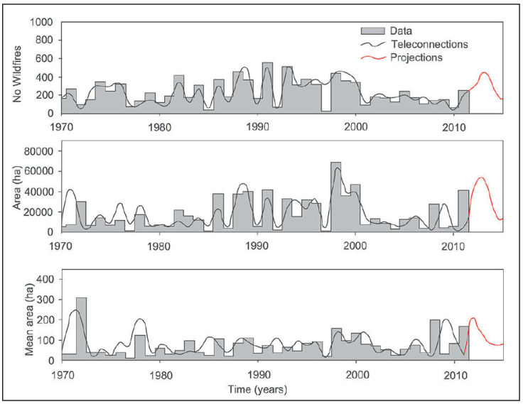
Figure 3 Modeling wildfire data using teleconnection regression equations coupled with local climate and soil data.
Other single independent teleconnection equations were reported previously by Návar (2011), as follows: A= 31600-12224ENSONOV_DIC-1, with an r2 of 0.37.
2. Autoregressive integrated moving average, ARIMA, models. All ARIMA models of the type ARIMA (1,0,0) in a log transformation data explained 48%, 45%, and 32% of the wildfire data set (No, A, AM, respectively). Examples of ARIMA models fitted to this data set are displayed in Figure 4.
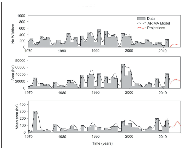
Figure 4 Autoregressive integrated moving average models projecting the number, the total area and the mean area burned by wild-fires in Durango, Mexico.
The advantage or disadvantage in rapid changing world climate extreme variability events, when using these stochastic models is that they can predict the future wildfire data with the same statistical properties as the original data set. Other ARIMA models using heterogeneous variance (ARCH and GARCH) had been recently developed that improve the predictability power for the time series with heteroscedasticity properties. However, the wildfire time series for Durango was tested for stationarity and independence and it is not long enough to show the likely heterogeneous variance that must have the high-severity in contrast to the small-severity wildfires and to fit the new ARIMA models. Other composed ARIMA models in conjunction with explanatory variables that may lead to the development of parametric models are under development and they will become better prediction techniques once they are tested and become available in the near future.
3. Regression equations. Annual, seasonal or weighted rainfall, evaporation, mean seasonal soil moisture content or the number of dry days during the dry season have been associated with some degree of confidence with forest wild-fires. Using the single most representative climatic station of El Salto, Dgo., Mexico (2570 masl), regression equations associated with wildfires are reported in Table 3.
Table 3 Degree of association between wildfire variables and several micro-climatic variables for the State of Durango, Mexico.
| Variable | Coefficient of Determination (r2) | |||
|---|---|---|---|---|
| X = θ | No | A | AM | |
| Number of Days with soil moisture content below θx | 0.29 | 0.15 | 0.23 | 0.18 |
| 0.31 | 0.14 | 0.23 | 0.18 | |
| 0.33 | 0.11 | 0.19 | 0.17 | |
| 0.35 | 0.13 | 0.22 | 0.18 | |
| 0.37 | 0.13 | 0.21 | 0.18 | |
| 0.39 | 0.12 | 0.21 | 0.17 | |
| 0.41 | 0.11 | 0.19 | 0.16 | |
| θ (Jan-Jun) | 1-6 | 0.22 | 0.44 | 0.33 |
| θ (Jan-May) | 1-5 | 0.24 | 0.32 | 0.21 |
| θ (Jan-April) | 1-4 | 0.26 | 0.33 | 0.20 |
| θ (Jan-March) | 1-3 | 0.30 | 0.60 | 0.21 |
| θ (Jan-Feb) | 1-2 | 0.29 | 0.33 | 0.17 |
| Annual Precipitation | P | 0.00 | 0.00 | 0.04 |
| Annual Evaporation | EV | 0.03 | 0.10 | 0.07 |
| Annual Evapotranspiration | ET | 0.01 | 0.01 | 0.04 |
| Dry Season (Jan-May) | P | 0.36 | 0.47 | 0.27 |
| Dry Season (Jan-May) | EV | 0.07 | 0.14 | 0.08 |
| Dry Season (Jan-May) | ET | 0.12 | 0.16 | 0.09 |
Note: These related variables are derived from a single climatic station while the number and area burned by wildfires is for all the State of Durango, Mexico. The number of days with soil moisture content below θx value, the mean soil moisture content, θ, Evapotranspiration and Real Evapotranspiration were modeled using a water balance budget approach. Data estimated for a single climatic station at El Salto, Durango, Mexico.
These local variables have a low to medium predictive power as the r2 hardly exceeds 50% of the wildfire variance.Of importance is the variable spring θ that is associated to the moisture content of fuels as well as the weighted Et component that is associated with both the heat and water available in the forest ecosystem. In case of using combined exogenous variables, the solution to the problem of heteroscedasticity relays on developing single, independent equations that predicts e.g., the A= (3170Exp(0.089/(θJAN-MAR-0.2451)); r2=0.60 that would yield more reliable predictions (Návar, 2015).
Using monthly temperature and precipitation data from other climatic stations located across the SMW mountain range, we developed multiple linear regression equations reported in Table 4.
Table 4 Multiple linear regression equations developed to predict wildfire data using climatic data from several stations placed across the Sierra Madre Occidental Mountain Range of Durango, Mexico.
| Wildfire Variable | Variable | R2 | N |
|---|---|---|---|
| A | Exp(2.68+0.037ATxJAN-0.1424STnFE-0.4217ATnMAR+0.215APMAR) | 0.59 | 29 |
| No | Exp(2.43+0.189ATxJAN-0.0038SPMAR+0.043TTnJAN+0.053T- TxFE) | 0.49 | 38 |
Where: A=Altares, b S=El Salto, T=Tarahumar, Tx=Maximum Temperature (°C), 18 Tn=minimum temperature (°C), P=monthly precipitation (mm), JAN=January, FE=February; MAR=March.
The use of instrumental climate data from other climatic stations increase prediction power of wildfires by accounting for nearly 50% of the total wildfire variance and having more stable statistical coefficients stressing the localized nature of wildfire at several times in the past and hence the aggregated nature of wildfires, as proposed earlier (Perez-Verdin et al., 2014). A potential geographical escalation could be also part of the prediction of wildfire regimes as drought develops seasonally quite frequently in latitude, longitude and altitude (Vega-Nieva et al., 2019).
B. Probabilistic Models.
1. Probability density functions. Examples of three pdf’s fitted in addition to the goodness of fit to each of the three wildfire variables are displayed in Figure 5.
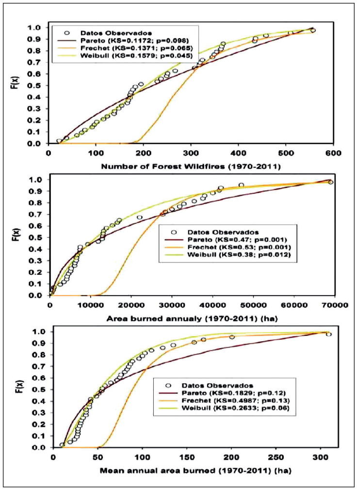
Figure 5 Three probability density functions fitted to the number of wildfires, the total area burned and the mean area burned in the State of Durango, Mexico.
The Kolmogorov-Smirnoff, KS, goodness of fit statistic is also embedded into each of the figures. The Truncated Pareto is an excellent model for high-severity wildfire data but fails to describe well the small-severity ones. The Weibull pdf function consistently models better all three sources of wildfire information. When using the Chi2 fitness statistic, the Weibull pdf tests the null hypothesis (P > Chi2 = 0.22; 0.12; and 0.16) of significantly describing well No, A, and AM, respectively.
The simulation of time series using random numbers retains the statistical properties of the original pdf and eventually produces similar values. The probability of high-severity burned areas (e.g., A > 20,000 ha) remains the same year after year. For this example, P(A>20,000 ha) = 31.67% for the original as well as for the simulated series. These results are important for the long term planning of the management of wildfires in the area of interest. However, they have little year to year predictive power unless the pdf is used within certain boundaries and coupling with other Bayesian techniques. For example, for these time series wildfire variables are related to each other (No = 1.9494Area0.4924; R2=0.66; AM = 0.513Area0.5076; R2=0.67) aiding in the prediction of the total area burned larger than 20,000 ha that could be of interest in forest fire management. Using the power regression equations reported above; this burned area is produced by about 255 wildfires with a mean burned area of 78 ha per wildfire. Using the Weibull pdf, there is a 31.67% of probability of any given year to have a burned area larger than 20,000 ha and it has therefore a probability of 68.33% of having a burned area smaller than 20,000 ha. Conditional probability would also eventually enhance prediction capabilities with the use of probabilistic models. The dependence of the probability on the explanatory X variables has been proposed in several statistical packages and they will eventually become techniques of wide acceptance and usage as the predictive power increase.
Assuming the Weibull pdf is a good model for the burned area; the generation of random values using this pdf function would provide predictions of past, present and future wildfire data. In this exercise using a simple Monte Carlo analysis generated 100 sets of 51 values (1970-2020) with the aim to use the series that correlates better with the measured wildfire data for the State of Durango, Mexico. Results are displayed in Figure 6.
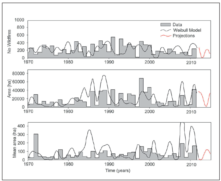
Figure 6 Measured and simulated random wildfire area data using Weibull probability density functions for northern temperate forests of Durango, Mexico.
The simulated burned area time series retains the statistics (e.g., for the mean burned area; mean = 20189 ha; standard deviation = 18373 ha; skew coefficient = 1.27) in contrast to the original measured time series (mean = 17753 ha; standard deviation = 15925 ha; skew coefficient = 1.18). The predictive power of these probabilistic models decrease in contrast with the ARIMA models (r2 ≤ 0.45) using a single realization of random numbers. Stronger Monte Carlo simulations may or may not improve the predictive power but they will probably extract better the true probabilities as well as any tendencies if any that would yield most robust likely future scenarios.
2. Markov chain matrices and models. For 2 states 1 was the burned areas of less than 20,000 ha and 2 burned areas larger than 20,000 ha. For 3 states; 1, 2 and 3 states could be for burned areas of less than 15,000; 15,001 ≤ 29,999; and ≥ 30,000, respectively.
The transition probabilities and their convergence matrices for two and three states for the total burned area are displayed next.
and
Both types of matrices for 2 and 3 states coalesce rapidly at steady state showing the stationary and the independence of the burned area time series. That is, for a Markov chain process with two states, the probability of shifting from a small-severity burned area (< 30,000) to a high-severity one (e.g., >30,000 ha) is exactly the same as if the process shifted from a high-severity burned area (>30,000 ha) to a small-severity one (<30,000 ha). For the 3 states Markov chain process, the steady state probabilities are also exactly the same for shifting back and forth from <15,000 ha; 15,0001 ha ≤ x ≥ 29,999 ha; and to ≤ 30,000 ha, respectively.
Future predictions of the area burned can be conducted using the three states matrix if for one moment it is assumed wildfires are not independent year after year by observing the area burned e.g., in 2012 (51626 ha; State = 3), the probability that A≤ 30000 ha in 2013 is then 99%; the probability that A ≤ 15000 ha in 2013 is then 72%; and the probability that 15000 ≤ A ≤ 30000 ha in 2013 is then 28%. The probability of the occurrence of wildfires with A ≥ 30000 ha in 2014 is 22%.
3. First order Markov Model. Measurements and predictions of wildfire data using a first order Markov model is depicted next in Figure 7.

The first order Markov model provides moderate (0.44 ≤ r2 ≤ 0.47) predictions comparing the goodness of fit statistics of the ARIMA models. A second advantage of Markov models is that they retain the same wildfire statistics (average, standard deviation, skew coefficient) as those of the original, measured data sets.
Short term wildfire predictions
Four single examples of measured and simulated wildfire data using five years of wildfire data set aside for validation of mathematical techniques is displayed in Table 5. The final row shows the coefficient of determination of the measured versus the predicted wildfire variables for each of four different prediction techniques.
Table 5 Validation of four mathematical techniques to predict wildfire data for the State of Durango, Mexico.
| Measured Data | ARIMA Models | Weibull pdf | Markov Model | Tele-connections | |||||||||||
|---|---|---|---|---|---|---|---|---|---|---|---|---|---|---|---|
| Year | No | A | AM | No | A | AM | No | A | AM | No | A | AM | No | A | AM |
| 2012 | 270 | 22802 | 84 | 308 | 43705 | 149 | 373 | 37352 | 11 | 446 | 10376 | 4 | 200 | 42005 | 210 |
| 2013 | 231 | 12359 | 54 | 251 | 6893 | 3 | 10 | 26273 | 16 | 273 | 4891 | 109 | 450 | 53000 | 118 |
| 2014 | 199 | 5463 | 27 | 74 | 39541 | 118 | 224 | 2268 | 121 | 190 | 13323 | 1 | 300 | 25000 | 83 |
| 2015 | 68 | 517 | 8 | 347 | 1933 | 6 | 97 | 35417 | 66 | 396 | 17567 | 13 | 160 | 13323 | 83 |
| 2016 | 254 | 7277 | 29 | 635 | 53403 | 84 | 43 | 22219 | 30 | 197 | 9800 | 0 | 340 | 45000 | 132 |
| R2 | 0.03 | 0.13 | 0.24 | 0.07 | 0.13 | - 0.40 | 0.05 | -0.33 | 0.05 | 0.25 | 0.43 | 0.78 | |||
The teleconnection technique using large scale as well as local hydroclimate exogenous variables provide more consistent results when validating the proposed equations (Table 5). However, large errors are expected when contrasting predictions with independent measured values left aside for validating models (Table 5). Most likely, using the properties of the Central Limit Theorem an average statistic using all available model predictions presented in this report would most likely improve assessment of the number or the area burned by wildfires in contrast to any single prediction equation by any mathematical approach tested in this report. This procedure would improve only average but not the extreme values that are important for the prediction of high-severity wildfires. As we are often interested in wildfire events such as those measured in 1998 during the strongest El Niño event of the last Century, other kinds of models must be developed to capture the variance of these high-severity wildfires.
Proposed New Models.
C. Physically-based models. More physically-based models should count for by the deterministic prediction of the three main components of forest wildfires; fuels and their moisture content, sources of ignition, and oxygen.
Fuels. Reinhardt and Crookston (2003) classified forest fuels as ground (organic soil, duff, and moss), slash (litter), living trees and miscellaneous (grass). These forest fuels can be further classified into: (i) litter, (ii) necromass, (iii) tips & stumps, (iv) branches, (v) foliage, (vi) living aboveground biomass. Litter has its origins in litter fall while foliage in the mass of leaves left on-site during harvesting operations.
Modeling litter and necromass stocks. Evaluations of forest fuel loadings on the forest floor conventionally measure altogether organic soil, duff, moss, litter and necromass.
Litter stocks. A physical model that predicts litter stocks and accumulation rates as a function of total aboveground biomass, the rate of losses weighted by site productivity was proposed for northern non-industrial reforested stands of Mexico (Návar, 2019). The physically-based model predicts cumulative litter stocks, LS, in growing forests. The model is parameterized using a mass balance budget approach as described below;
The final model is described in Eq. [4] and Eq. [5], as follows:
Where: LR = litter fall rate (Mg ha-1y-1); LO = rate of litter losses (Mg ha-1y-1); LS = litter stocks (Mg ha-1y-1); AGB = aboveground biomass (Mg ha-1); P, ET = mean annual precipitation and Thornthwaite evapotranspiration, respectively (L).
The litter stock and accumulation model was previously validated with measured litter stock data for local Mexico’s forests (Renteria et al., 2005; Acosta-Mireles, 2003; Rodríguez-Laguna et al., 2009; Mendoza-Ponce & Galicia, 2010; Aryal et al., 2018; Caballero-Cruz et al., 2018), as well as for average data reported for Mexico (CONAFOR, 2012), North American (Kohl et al., 2015) and World (Kohl et al., 2015) temperate forests (Figure 8).
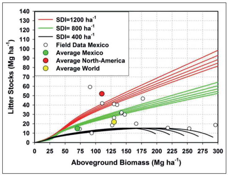
(Source: Navar, 2019)
Figure 8 Modeling litter stocks & accumulation rates using a mass balance litter budget approach for northern temperate forests of Mexico coupled with a whole stand growth and yield model with three stand density scenarios.
Necromass: tree mortality by competition. Tree mortality is the main source of necromass accumulating atop the forest soil. Tree mortality occurs by competition and by stochastic processes. Tree competition can be predicted using the conventional technique of mortality by demography, as competition for space and resources is the main driver of tree mortality in overstocked forests and plantations. Overstocking develops in forests as trees grow in size. The Reineke equation predicts quite well tree density as a function of mean diameter, with a typical log-log relationship and the universal exponent of -3/2 ensures the reduction of the number of trees as they grow in diameter. Using this principle, an equation evaluating stand density, Den (No ha-1), is developed. In this example, using available data for North American forests, the Den Eq. was developed, as follows;
Where: Den = stand density (No ha-1); D = diameter at breast height (L).
Fortunately Eq. [6] reproduces similar Den data as the equation reported by Aguirre-Bravo (1987) for Pinus cooperi stands of Durango, Mexico. Then, the number of trees dying by competition was evaluated using Eq. [7],
The total number of trees killed by competition at t=t is evaluated using Eq. [8],
Using the diameter growth Eq. (D = f(T)) described by the sigmoid Chapmna-Richards function for local forests (Corral-Rivas and Návar-Cháidez, 2005); the Den = f(D) by Eq. [6], as well as the AGB =f(D) equation for individual trees reported earlier (Návar, 2009), we derived the cumulative AGB of killed trees by competition that are eventually aggregated to the forest floor as the main necromass input. Figure 7 presents the AGB density of killed trees by competition.
The annual tree mortality rate by intrinsic competition has an average of 2.0 Mg ha-1y-1. As expected it is more acute in the most productive forests. In temperate forests of Durango, Mexico, high-severity wildfires present an average frequency of approximately 30 years (Rodriguez-Trejo and Fule, 2003; Drury and Veblen, 2008) and using this information, under no management practices of on-site killed trees by competition, this forest would accumulate an average of 60 Mg ha-1. However, because necromass has a half life time in the environment of 20 years as it decays over time; the final necromass density would be in the range of 20 to 30 Mg ha-1 during any average time interval between two consecutive high-severity wildfires.
Tree mortality by random processes. The forestry institutions over the world report forest inventories with the number and volume of dead on-site trees. For Mexico, the CONAFOR (2012) reports the total annual volume of harvested dead on-site trees, with a mean of 50,000 (±10,000) Mg. However, the total volume of dead on-site trees is approximated in the forest inventory and this volume can be sometimes twice as large as the total official harvested timber volume. For example, Návar (2015) reported two important episodes (1998-2001 and 2012-2012) that killed on-site large number of trees by a combination of infrequent drought-related disturbances with heat waves, frosts, wild-fires and bark beetle outbreaks. Official reports recorded an area affected of nearly 200,000 ha by these disturbances in each of these two dry spells that may have accounted for a standing biomass of approximately 1 M Mg.
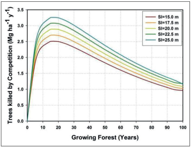
Figure 9 Quantifying the aboveground biomass density input of trees killed by competition in northern native forests of Durango, Mexico.
The rate of tree mortality in the presence of other stochastic processes such as frosting winds, strong cold-dry winds, pests & diseases, drought spells associated with heat waves, among others require further attention since these stochastic events add large amounts of fuels in the form of litter and necromass to the forest floor. This explains why in some regression analysis, the minimum extreme temperature explains a significant portion of the large wildfire variability as it was the case for the data set of in Durango, Mexico. Unfortunately the data base comprising these random events is non-existent or at least a couple of data points in time are available making developed models to have a limited predictive power. More efforts are required to enriching the data base using paleo climate & historic wildfire data techniques.
Other forest management practices producing forest fuels Forest fuels as residues of conventional forest management operations. Timber harvesting also add considerable mass of litter, branches, stumps, and tree tops on the forest floor that can be predicted in advance quite well. Most of the stem component is harvested, with the exception of stumps, branches and tree tips. With the use of taper functions, the stem can be partitioned into merchantable or harvestable and non-merchantable or non-harvestable components. Most branches and all foliage components are usually left on site. With the use of aboveground biomass allometry, the mass of branches, foliage and timber stump & top components can also be predicted in advance.
Timber stumps & tips left on-site. Timber stumps are the basal portions of the main bole left standing on site. Timber tips are the distal portions of logs that do not meet the size requirements for its transformation into merchantable components. They are sometimes collected for the transformation of secondary forest products and sometimes they are left on-site as well. Mathematical functions that predict the stem profile had been developed over the years for many forests. An example for northern temperate tree species of Mexico reported by Návar et al., (2013) is presented next. The equation of Newnham (1990) depicted by Eq. [9] with recorded parameters for local pines and oaks (Table 6) predicted total, merchantable, stump and tip volumes.
Where: H = top height (m); hi = relative height (m); D = diameter at breast height (cm); d = relative diameter (cm)
Table 6 Coefficients of the Newnham (1990) taper model and their standard errors for tree species of northern Mexico.
| Parameters | |||
|---|---|---|---|
| Species | Statistic | b1 | b2 |
| Quercus spp | Mean | 0.010400 | 0.916300 |
| SE | 0.000036 | 0.011100 | |
| Pinus spp | Mean | 0.010300 | 0.595400 |
| SE | 0.000017 | 0.003200 | |
Source: Návar et al., (2013).
The difference between total, Vt, and merchantable, Vc, timber volume evaluated the timber tip volume, Vtt, as explained mathematically by Eq. [10], as follows:
Equation [10] cannot be analytically integrated, hence numerical analysis is conducted, e.g., using δhi=1 cm. Merchantable timber was evaluated from the base to the length of stem where diameter is > 20 cm. Logs with D ≤ 20 cm are classified as tips. Tip biomass was estimated by multiplying the tip volume times its wood specific gravity. Timber stumps are calculated using conventional empirical equations.
Branch biomass. Branch biomass of harvested timber can be quantified using allometric equations that have also been developed for many tree species for many forests. Návar (2009) reported for northwestern forests branch biomass equations for pine, Bbp, and oak, Bbq, tree species. These equations are:
Where: dry biomass is in kg; D = diameter at breast height (cm).
Using this approach, the mass of fuels that remain in the forest floor is approximately 3 Mg ha-1y-1. An example of the calculations using the Newnham (1990) equation at the stand scale is reported in Table 7.
Table 7 Statistics for classifying biomass components of 62 overstocked stands of northern temperate, mixed, uneven-aged forests of Central Durango & Southern Chihuahua, Mexico.
| Total | Tree Tips | Stump | Biomass Components (Mg ha-1) | |||||
|---|---|---|---|---|---|---|---|---|
| Branch | Foliage | Necro- mass | Sawnwood | Plywood | ||||
| Mean | 171.8 | 23.0 | 6.9 | 34.3 | 20.6 | 24.2 | 76.1 | 41.6 |
| Standard Deviation | 71.7 | 11.6 | 2.9 | 14.3 | 8.6 | 14.5 | 40.5 | 39.3 |
| Confidence Interval | 17.8 | 2.8 | 0.7 | 3.5 | 2.1 | 3.6 | 10.0 | 9.7 |
Evaluations of biomass components of Table 7 assume all trees are harvested in these forest stands. This is of course not possible as clear cutting practices are forbidden by the Mexican Forestry Law. Then, ratios can be used to predict the biomass components left on the forest floor as a function of the allowable harvest. These ratios must also be weighted by the half life in the environment of each forest fuel component.
Live trees. Live trees become also important sources of forest fuels especially when they reach very los internal moisture contents (< 7%). The aboveground biomass contained in standing live trees can be evaluated using already developed allometric regression equations. A wide range of allometric equations at the species and temperate species were developed and reported by Navar (2009) that were applied to the Mexican Forest Inventory for Durango, Mexico. An example of this approach is presented in Figure 8 where close to 1700 forest inventory sites are displayed.
The climatic component. The moisture content of forest fuels is the single most important hydro-climatic component controlling wildfires because depending on the fuel water content the wildfire can simulate a prescribed burn, a small-severity or a high-severity wildfire. Due to the difficulty of continuously measuring and evaluating the moisture content of fuels, numerous climatic indices have been proposed with little predicting power; e.g., see statistics of Table 3.
The moisture content of forest fuels. The moisture content of forest fuels (ground, litter, grass, trees) can be deterministically evaluated using several approaches. Návar (2015) assumed the soil moisture content is in equilibrium with the forest fuel moisture content as they are in close contact and developed a physical water balance budget model to evaluate changes in soil moisture content, δθ, over time, δt, that is depicted by the next set of equations.
Where: In = water inputs (L); Ou = water outputs (L); θ = soil moisture content (L L-1); P= precipitation (L); I C,LS = Interception loss of forest canopy and litter, respectively (L); E V = Pan evaporation (L); T R = transpiration (L); Q S = Surface runoff (L); Q SF,AR = Subsurface runoff and aquifer recharge (L).
Making several further assumptions, the θ is evaluated with very good preliminary expectations as it correlates well with wildfires (0.34 ≤ r2≤ 0.95); tree growth and productivity (0.40 ≤ r2≤ 0.50); pulses of tree dieback (0.34 ≤ r2≤ 0.50) (Návar, 2015). In fact, the best prediction equations of Tables 2 and 3 include θ as the most significant explanatory variable. However, Návar (2015) has found the predictive power of θ weakens as the wildfire time series data lengthens.
D. The proposed conceptual model. Wildfires are associated and significantly synchronized but complex manner with SST oscillations (ENSO, PDO, and AMO) because other local variables such as the availability of fresh foliage and its moisture content also contribute to set the right environmental conditions to unleash these perturbations. Extreme Ocean temperatures beyond average values, dT, are well associated with high-severity 1wildfires and this effect magnifies when all three major SST (ENSO, PDO, AMO) 1anomalies converge over time. As the Oceans warm, the heat waves would eventually 1reach the continents and forest ecosystems, which are from Holartic origin, suffer the consequences through a series of perturbations where the increasing frequency of high-severity wildfires is just one of them.
The ENSO disrupts world climate and it has a profound influence on the precipitation and temperature in many places on Earth, as it is the case for Mexico (Cavazos y Hastenrath, 1990; Méndez-González et al., 2008). In the presence of ENSO, Northern Mexico shifts climate in winter and spring to wetter and colder that correlate very well with the southern displacement of the Lower Aleutian convergence zone in the Northern Pacific Ocean in combination with a stronger Inter-tropical Convergence Zone jet stream of the Central Pacific Ocean (Andrade y Sellers, 1988). Swetnam y Betancourt (1989) in California & Arizona; Drury and Veblen (2007) and Návar (2011) in Durango, México noted the weak but significant synchrony of wildfires with ENSO t+1 events. Due to these conditions, at ENSO t=t, soil moisture content also becomes wetter reducing the risk of high-severity wildfires to nearly 0 and increasing forest productivity (González-Elizondo et al., 2005; Arreola-Ortiz and Návar-Cháidez, 2010; Návar, 2011; 2015).
The joint effect of ENSO, PDO, and AMO on wildfires combines to produce more complex environmental settings (Fig 10). A further explanation of the conceptual framework is given next. These SST oscillations appear to unleash a chain of large-scale bio-climate anomalies in northern forests of Mexico as follows: (i) warming of the Eastern South-Central Pacific Ocean (ENSO, t=t) strengthens Arctic Westerlies (PDO is a good signal) bringing unseasonal winter and spring below average temperatures and above-average precipitation; (ii) as the warm ENSO (t=t+1) Eastern Pacific Ocean current displaces north and arrives in Mexico temperature shifts to above normal and precipitation to below normal that last until the warm Ocean Current migrates or vanishes over time or La Niña takes over the Equatorial Pacific Ocean temperatures; (iii) next seasonal winter and spring climate feature unusual flashy northwestern Ocean waves of frosting air masses or dry flashy intermittent strong arctic cold front systems entering the country controlled partially by the PDO anomaly and probably given by the difference in Ocean temperatures where the two Pacific Ocean currents (ENSO and PDO) meet promoting leaf senescence of frosted foliage of several forest species and adding important amounts of fresh foliage to the forest floor; and (iv) in the presence of a warm-phase AMO, warm Eastern Atlantic air masses (easterlies) arrive in late winter and early spring with air temperatures that depend on the AMO signal and the Gulf Current temperature. Combined warm Equatorial Pacific and Atlantic Ocean currents would bring higher than normal temperatures to the country. Hotspots are good indicators of the convergence of AMO and the Gulf Currents. In addition to high temperatures, the Bermuda-Azores anticyclone strengthens creating the ideal conditions that inhibit precipitation magnifying further the dry spell in most of northern Mexico. Figure 12. The conceptual model for predicting high-severity wildfires in northern forests of Mexico.
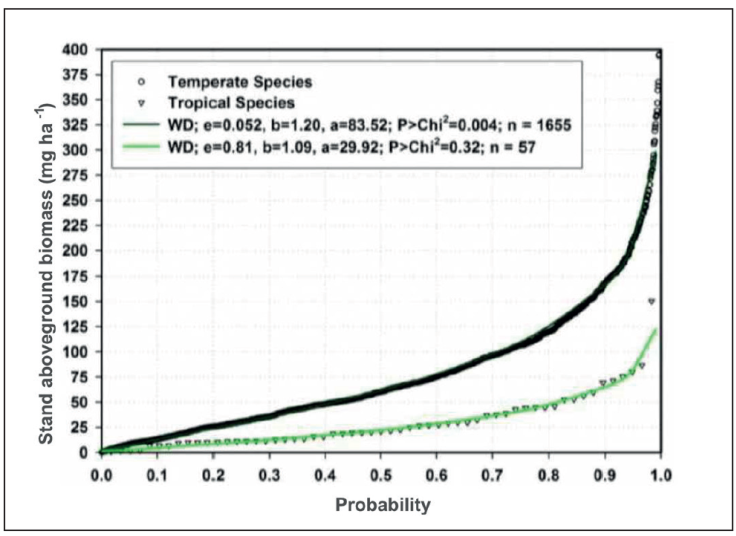
Figure 10 The aboveground biomass density for nearly 1700 forest inventoried sites of Durango, Mexico.
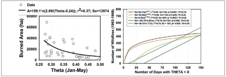
Figure 11 Predicting wildfire data with predicted soil moisture content for temperate forests of Durango, Mexico.
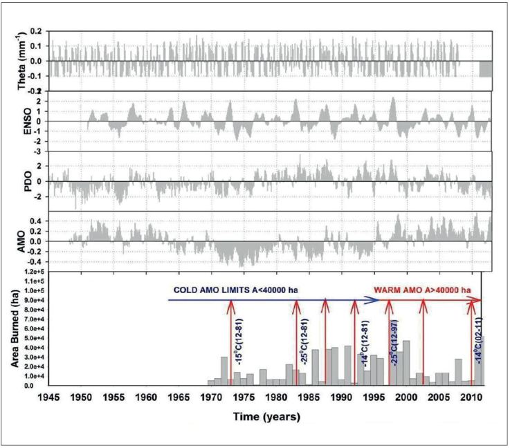
Figure 12 The conceptual model for predicting high-severity wildfires in northern forests of Mexico.
Intense flashy frosts usually make several tree species shed an important part of the foliage in the course of weeks; adding important amounts of biomass composed of fresh foliage and branches to the forest floor (Rocha-Loredo and Ramírez-Marcial, 2009; Návar-Cháidez and Jurado-Ybarra, 2009). Warm easterlies temperatures further desiccate fuel loads; set erratic hot-temperature waves of air masses (promoting hotspots in forests) further weakening live forests and frequently promoting tree die off increasing further on-site fuel loads (Allen et al., 2010; Raffa et al., 2010; Návar, 2015). The dry spell intensifies and magnifies in spatial extent drying further any additional fuel load including live trees, shrubs, forbs and grasses. This scenario has repeated several times in the past and set free the presence of important high-severity wildfires in Northern forests of Mexico. Note that when the AMO is in a cold phase (1970-1995), the burned area by wildfires hardly exceeds; A ≤ 40,000 ha; in contrast to when it is in a warm phase; A>40,000 ha. Same thing happens to the intensity or failure of each or both the ENSO and PDO anomalies that control part of the wildfire variability. This is the partial reason why any of these SST anomalies alone would account for only a small portion of the wildfire variance.
Wildfires are then a complex function of several bio-climatic processes that can be modeled using most of the mathematical techniques described above. The cycle may start from: (i) modeling the future ENSO anomaly using the conventional ARIMA techniques, large-scale climate models, or NOAA reports; (ii) model the fuel load using the physical model proposed above as well as using the probabilistic or stochastic techniques, yet to be developed, to evaluate the effect of unusual intense frosts (associated with PDO) and hot temperature waves of air masses (associated with AMO) on fresh fuel loads; (iii) use the physical hydrologic mass balance budget model whenever possible to predict the moisture content of the fuel load itself (yet to be developed) or of the forest soil to predict dryness of fuel loads (see Návar, 2015), including the moisture content of live forests; and (iv) prepare for the worst-case scenario by using all the information available.
Discussion
The right hydro-climate conditions that promote high-severity wildfires recorded in the historic data set prevailed in Durango during the most intense ENSO event of the last century (1997-1998) (dT ≥ +2.45°C); combined with AMO (dT ≥ +0.50C) and PDO (dT ≥ +2.0°C) anomalies that caused the record statistic of burned area in Durango (A ≥ 80,000 ha), as elsewhere in the world. These environmental conditions persisted across most forests of the country (CONAFOR, 2012; FAO, 2012). The long-term cycle for the AMO to repeat is from 60 to 80 years (Einfeld et al., 2001); 24 years for the PDO (Mantua, 1999) and 3 to 7 years for the ENSO anomaly (Cavazos and Hastenrath, 1990). The AMO is currently in the warm phase that started in 1997 (https://www.esrl.noaa.gov/psd/data/correlation/amon.sm.long.data). The warm phase will likely continue its normal cycle for the next 10 to 15 years dumping warm and probably hot air masses from the Equatorial Atlantic Ocean and strengthening the anticyclone Bermuda-Azores sharpening dry spells with associated hot air masses. Using data from NOAA-US (https://ggweather.com/enso/oni.htm), the ENSO is not relaxing; it is in fact fortifying over time as the maximum Eastern South-Central Pacific Ocean temperature deviances, expressed as the Ocean El Niño Index, ONI, are significantly increasing over 31 time: 1957-1958 (dT=+1.7°C); 1965-1966 (dT=+2.0°C); 1972-1973 (dT=+2.05°C); 1982- 32 1983 (dT=+2.25°C); 1997-1998 (dT=+2.40°C); and 2015-2016 (dT=+2.60°C). However, the ENSO long-term cycle is yet to be assessed and the most likely future scenario would be to assume it will continue its rising trend in the years to come. If so, rising seasonal extreme temperatures and precipitation events are expected in the short run as it reinforces the temperature gradient between the arctic and the equatorial Western Pacific Ocean as well as supporting increased temperatures of the ENSO current moving northward across the shoreline of the western coasts of tropical America. The PDO is developing more erratically in modern times (https://www.ncdc.noaa.gov/teleconnections/pdo/) from 2005 to 2014 was in a cold phase then it entered into a short warm (2015-2017) to return to a cold phase again (2017-2019). Short-term predictions would be to assume this erratic trend will likely continue.
Under this short run future scenario, northern forests of Mexico would probably experience the most severe wild-fires yet to be recorded in modern times in the next 3 ENSO events (20 years) because of the joint presence of extreme positive ENSO and AMO anomalies. However, intensification of high severity wildfire could be limited by only the erratic PDO anomaly should it be in a cold phase when the warmest ENSO and AMO climate signals meet in the near future. However, as the AMO would enter into a cold phase in the next 15-20 years, should the anomaly follow its normal track (returning to below average temperatures), after 30-40 years of a warm phase (Einfeld et al., 2001) wildfire severity would most likely relax returning to a kind of normal severity, A<40,000 ha (See Fig 10 of the wildfire data during the cold phase of AMO). The cold-phase PDO keeps normal or below-average temperatures over Western North America dumping seasonal erratic infrequent cold air masses over Northwestern Mexico in winter and early spring. The partial PDO effect on wildfire can be exemplified next. In spite of this rising trend in temperature deviance, the wildfire severity peaked during the 1997-1998 ENSO event (A≥80,000 ha) even though the 2015-2016 (A=40,000 ha) ENSO event exceeded the temperature deviance of that of 1997-1998. This contrasting finding is explained by the sudden weakening of the PDO entering shortly into a cold phase in 2017-2018. Other factors that may have contributed to keep wildfires in check could be a lack of fresh foliage caused by the absence of extreme cold temperatures; forest fuels were not dry enough; among others. This is a matter of further research in order to forecast the severity of wildfires of the following ENSO events.
Conclusions
This report presents, tests and validates a series of mathematical techniques to predict in advance wildfire data at regional scales. Stochastic and probabilistic models provide from medium to moderately well prediction capabilities. Proposed physical and conceptual model are underway and would probably become the next generation of models that will eventually forecast with higher precision the likelihood of high-severity wildfires. These technologies, as exemplified in this report, predict better fuel loadings and the moisture content than conventional approaches and these techniques would eventually be coupled with the prediction of large scale SST anomalies that have a marked influence on a chain of bio-climatic events unleashing high-severity wild-fires in many regions of Earth. These events are proposed to be predicted in advance and coupled into the conceptual framework. These issues are a matter of further research.

