


 nova página do texto(beta)
 Inglês (pdf)
 Artigo em XML
 Referências do artigo
 Enviar este artigo por email
 Citado por SciELO
  Similares em
SciELO
Similares em
SciELO 
 Permalink
1.Introduction
The confinement and guidance of electromagnetic radiation in dispersive media due to total internal reflection is of great interest in many fields of theoretical physics, including radiative transfer in the Earth’s atmosphere and astrophysical media 2,3. Particularly, an extensive literature concerning the confinement and guidance of radiation in media with radially varying refractive index, usually called GRIN media, does exist. Research on these topics has allowed the design and manufacture of all kinds of devices that involve non-homogeneous media: integrated optics, lenses, waveguides, optical fibers, and diffraction gratings 4,5.
On the one hand, the confinement of radiation in non-homogeneous media with a given refractive index profile has been a highly researched topic. We ourselves, in two previous articles, (6),(7), PI and PII hereafter, have analyzed the captured radiation in systems where the refractive index, n, varies smoothly with r, the radial coordinate. Dealing with spherically symmetric systems in PI and with cylindrical symmetry systems in PII, we apply the Fermat’s extremal principle in the framework of the geometrical optics to analyze the confinement of the guided radiation in a given region. Analytical solutions of the ray-tracing problem can be found in 8-10. Also, Evans , by comparing the Newtonian mechanics with the laws defining geometrical optics, has calculated the three-dimensional trajectory of a ray propagating through a medium with a parabolic refractive index.
On the other hand, the reconstruction of the unknown refractive index profile of a waveguide according to the behavior that the radiation traveling through it shows is also a highly researched topic: from the first works using interferometric techniques through those based on the measurement of the evanescent field on the surface of the waveguide combined with the use of sophisticated algorithms (13 and references therein), to one of the newest proposing a non-destructive iterative interferometric tomographic technique .
At the present paper, we intend to analyze the confinement of radiation in waveguides useful in both directions: i) given the refractive index profile in the guide, to infer how the radiation will be guided according to the distance and the angle respect to the axis of the guide with which the radiation entered, and ii) knowing how the radiation travels along with the guide, to obtain information on the radial variation of the refractive index within it and how the radiation entered the guide.
Using the simple criterion we have established in PII that allows us to infer whether radiation confinement occurs in a given system, we intend to contribute to the design of waveguides for predefined objectives, emphasizing on the design of multi-mode guides. Multi-mode waveguides are built with either graded index or step-index. Graded index guides minimize modal dispersion, although they have the disadvantage of being more expensive and difficult to build than step-index guides. In this work, we will address both options.
We organize this paper as follows: In Sec. 2, we set out the basis of our work methodology. In Sec. 3, we analyze the confinement regions of radiation traveling through a waveguide in which i) n takes a constant value a little greater than 1, sharply dropping at the edge (Sec. 3.1) n has a series of steps (Sec. 3.2 and 3.3) n has a parabolic radial variation (Sec. 3.3). In Sec. 4, we address the inverse process, namely, to find the right refractive index profile of the waveguide to radiation travels confined in a given region. In Sec. 5, we present our conclusions.
2.Framework
In PII. we considered a homogeneous transparent cylinder of radius R and infinite length characterized by a refractive index n > 1. There, we considered a light ray propagating within the cylinder in an arbitrary direction, but no parallel to the cylinder axis, so that it eventually would strike the cylinder wall in which it would be reflected and refracted. The reflected light would continue traveling inside the cylinder until it again strikes the cylinder wall. If total internal reflection occurs, the process will be repeated over and over again. In Fig. 1 of that paper, that we reproduce here as Fig. 1 for simplicity, we showed the portion between P1 and P2 of that endless journey within the cylinder, being P1 and P2 the points in the cylinder wall where two successive reflections occur. We defined a Cartesian coordinate system so that the Z-axis is along the cylinder axis, the ray is on a plane which is parallel to the Y-Z plane, and the X-Y plane intersects the ray at P0, the point which is equidistant from P1 and P2.
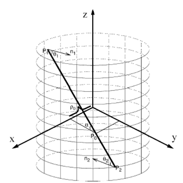
Figure 1 Used coordinate system. Coordinate system defined to describe the path of a ray of light in a system with cylindrical symmetry (see text for definition of the parameters).
Considering a system whose refractive index presents a monotonic variation with p,
the distance from the cylinder axis, and getting rid of the n dependence on v, the
light frequency, we have defined in PII two parameters that fully characterize a
given ray: i)
In PII, applying the Fermat’s extremal principle in the framework of the geometrical optics, we have shown that, in systems with cylindrical symmetry where the refractive index varies smoothly with the distance to the cylinder axis, confinement of radiation does occur, provided it is verified
This expression allows finding a two-dimensional domain defined by the parameters
For a given n(p), the confinement region is a region in the (
Now, we will take into account that the limiting curves of the confinement regions could be found by analyzing the Legendre transform of the function defined by the left hand of Eq. (1).
To comprise this, let us consider as an example n(p) given by the parabola
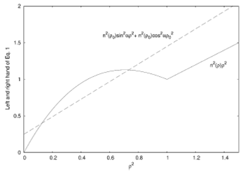
Figure 2 Left and right hand of Eq. (1). The left and right hand of Eq. (1) are shown as functions of ρ2 for given ρ0 and a values.
Although the maximum of the curve will not occur within the waveguide for
n0 values lower than 1.5, a confinement region will exist, and the
analysis we are going to do is quite the same. On the other hand, the right hand of
Eq. (1) is always a straight line whose slope and intercept depend on the
If n(p), rather than being represented by a smooth curve, exhibits a step on the edge of the guide, the curve displayed in Fig. 2 will increase monotonically with p2 until it reaches a maximum at p2 = 1 where it will abruptly go down. In this last case, at the same conclusions, we will arrive through a similar analysis.
Using the Legendre transform of the function y(x), instead of the function itself, to find the confinement regions gives us several advantages:
it allows us to make a general analysis, applicable in any case regardless of the particular form of n(p),
it gives us a new space of analysis easier to interpret and visualize, very convenient in the context of our task and
let us conclude straightforward manner about the characteristics that our waveguide should have so that the radiation is confined in one or another region according to our interests.
The equivalence of the analysis methods will be verified in the next sections by recovering the results we have reached in PII for the two n(p) functions we took as examples at that occasion, namely, one step and parabolic index. At that opportunity, we intended to find the confinement region for a given n(p). In the present paper, we also focus on developing the reciprocal process: to find the n(p) with which the waveguide should be built for a sought-after confinement region.
3.Looking for confinement regions for a given n(p) by using Legendre transform
The function whose Legendre transform we have to find is
where x = p2.
We intend to pass from the (x,y) to the (u, v) plane through the Legendre transform, doing
where u and v represent the slopes and intercepts of the tangent lines to y(x) .
Before continuing, we want to highlight two things. First, regardless of whether n(p) is a continuous and derivable function for any p value or not, we can always move from the (x,y) to the (u,v) plane by the appropriate considerations. The considerations we are going to do in the following sections to find the equations of the tangent straight lines to y(x) must be interpreted as a way of extending the concept of Legendre transform at the discontinuities. We must keep in mind that the discontinuities, in the context of a physical model of a continuous medium, represent only a very convenient mathematical simplifier alternative for the model. They do not imply, however, essential physical facts.
Second, regardless of the functional form of n(p), the slopes and intercepts of all straight lines that cut twice the curve representing y(x)are positive numbers, since all these lines are represented by the right hand of Eq. (1). This restricts the solutions to the first quadrant of the (u,v) plane.
4.Applications of the method
In this section, we aim to apply the methodology exposed in the previous section to particular cases. For the sake of looking for confinement regions by using Legendre transform, we will carry out the analysis for three different n(p), two of which were already analyzed in PII, namely: i) n(p)takes a constant value a little greater than 1 inside the waveguide and sharply drops to 1 at the edge of it, ii) n(p)has a series of steps inside the guide, characterized by a value of n(p), n i , each of them and iii) n(p) is a parabola.
4.1.One step index waveguide
Firstly, let us consider the simplest case: a homogeneous transparent cylinder of
radius R and infinite length, which is characterized by a refractive index
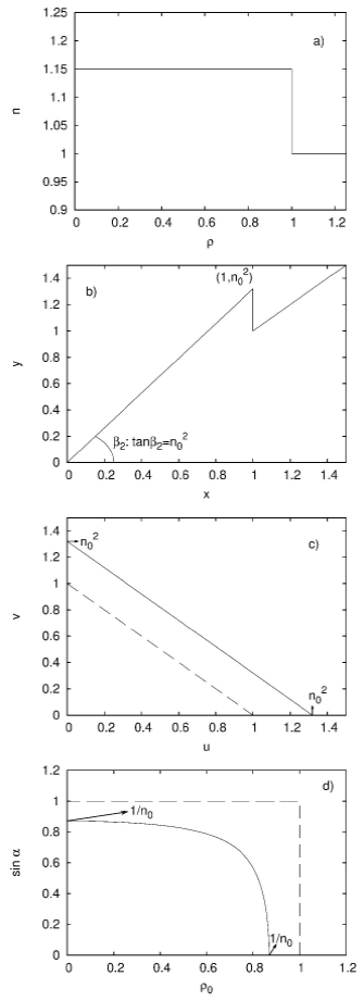
Figure 3 One step refractive index profile. For a system characterized by one step refractive, index we display: n as a function of ρ0 in panel a), y as a function of x in panel b), v as a function of u in panel c), and sin a as a function of ρ0 in panel d).
Since n(p) = n0 if p < R and n(p) = 1 if p > R, inside the guide Eq. 2 can be written as
We intend to find, first, the curves in the (u,v) plane that limits the zone of possible slope and intercept values of straight lines that cut y(x) twice.
Even though in the case we are considering y(x) is not a continuous function at x = 1, it is easy to get the results we are looking for by making the appropriate considerations.
Firstly, from Fig. 3b) it is easy to see at once
that any line cutting y(x) fulfill
By taking into account these considerations, it is straight forth to find that all the straight lines that cut the curve drawing in Fig. 3b) twice have a slope and intercept values in a region delimited by the two straight lines
and
being Eq. (6) the equation linking slopes and intercepts of every straight line
passing through the point
Taking into account that, in order Eq. (1) is satisfied, it must be fulfilled:
and
we finally obtain the limits of the confinement region in the plane
This region is shown in Fig. 3d), where it is
clear that varying n0 results in a variation of the size of the
confinement region: the greater n0, the greater the confinement region.
If the system, instead of being in the air, is a traditional waveguide consisting of
a core with
In PII, the results for a system characterized by a one-step refractive index were given in terms of x and z, being x the X coordinate of any point between P1 and P2 on the ray traveling inside the cylinder (since the ray is on a plane which is parallel to the Y-Z plane), and z the Z coordinate of P2. To show that the expression in PII, reproduced below for simplicity,
is equivalent to Eq. (10) in this paper, let us make the following considerations.
Firstly, since
4.2.Multi-step index waveguide
An extension of the previous case is the case for which n(p) presents, within the waveguide, a series of steps, rather than a single one. This is the case of multilayer cylindrical waveguide, of great interest for its possible technological applications. Guided radiation achieved by total internal reflection through multilayer waveguides has been analyzed in articles as . Some others, like 16, analyze the multilayer cylindrical waveguide structures by identifying the modal field excitations supported by the corresponding waveguide, regardless of the guiding mechanism.
The case we are considering is the simplest one: n(p) within the waveguide is
represented by an N steps stair, with equal height and wide all of them, as it
is illustrated in Fig. 4a) for N = 5. The
guide of our example, thus, consists of five regions, Ri, extended
from
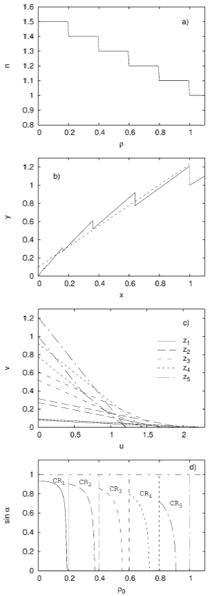
Figure 4 Multi-step refractive index profile. For a system characterized by multi-step refractive, index we display: n as a function of ρ0 in panel a), y as a function of x in panel b), v as a function of u in panel c), and sin a as a function of ρ0 in panel d). In panel b), a straight line with slope u1 and intercept v1 is also shown (see text).
Although y(x) exhibits discontinuities at every
From Eqs. (13), (14) and (15), and taking into account Eqs. (8) and (9), the
corresponding confinement regions in the
Each of the five zones in the (u,v) plane, Zi hereafter, corresponding to each
of the five teeth of y(x), is displayed in Fig.
4c). Therefore, Zi contains all the possible slope and
intercept values of the straight lines that cut the ith tooth twice.
Consequently, the different confinement regions in
However, it is apparent from Fig. 4c) that
the spaces of solutions in the (u,v) plane corresponding to the different teeth
of y(x) intersect each other. Taking into account expressions (8) and (9) that
allow the calculation of
But, even for values of (u,v) belonging to these intersections, radiation will always travel confined exclusively in one, and only one, a region of the guide, Ri.
On the other hand, outside these five zones Zi, there are (u,v) values for which the radiation remains confined in a sector of the guide, spanning, however, more than one single Ri region. Areas in the (u,v) plane limited by the straight lines given by Eqs. (13) and (14), but not (15), define a strip that differs from the space of solutions for a given tooth in a triangular area like the one labeled Area A in Fig. 5b), enlargement of Fig. 4c). Although the Area A corresponding to 4th tooth is the only one indicated in the figure, each tooth has its own Area A. Straight lines with slope and intercept values contained in Area A of the ith tooth will cut this tooth where it sharply drops and some other where it ramps upward. This leads to radiation being confined between the two corresponding regions of the guide.
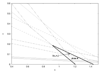
Figure 5 AreaA corresponding to the 4th tooth. AreaA corresponding to the 4th tooth (see text for definition) is highlighted in an enlargement of Fig. 4c).
Then, for reasons that will be clearer below, it is important to know how the
curves that delimit every confinement region CRi exhibited in Fig. 4d), defined for
To get curves defined for all
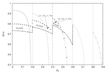
Figure 6 AreaB corresponding to the 4th tooth. The AreaB corresponding to the 4th tooth (see text for definition) is included in an enlargement of Fig. 4d).
To make things clearer, let us take as an example the point
At the same conclusions, we should arrive by analyzing the solutions in the
For another point
where
Clearly, it is possible to do this for any other point
Finally, for the sake of clarity, a generalization of the results we have achieved in this section is written in the following two paragraphs.
On the one hand, going from (p,n) plane to
On the other hand, from Fig. 7 where the five Area B
i
are exhibited along with the five
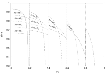
Figure 7 AreaB for the five teeth. sin a as a function of ρ0 is displayed as in Fig. 4d) but including the curves that delimit the AreaB for the five teeth.
4.3.Parabolic index waveguide
In PII, we have also considered as an example of a system with a parabolic variation of refractive index. Waveguides with 𝑛 varying this way, first developed by Uchida et al. 17 and named SELFOC®, is of great interest since it has been shown that a parabolic radial variation of the refractive index considerably decreases distortions and losses. For that reason, it is widely used in optical communication and data processing.
In this case, n(p) can be written as
having n0 and A the meaning we have set in Sec. 2. For different A
values, we have found in PII the confinement regions in the
At the present paper, for n(p) given by Eq. (24), we start writing Eq. (2) as
to move from (x,y) plane to (u,v) plane through the Legendre transform.
Then, through Eqs. (3) we obtain
and
Replacing Eqs. (27) and (26) in Eq. (4) and taking into account the Eq. (25), we obtain:
According to its definition, A can be calculated as
where n1 is the refractive index of the surrounding medium of the system. If the system is in the air, we can set n1 = 1, and Eq. (28) becomes a function of u and the n0 parameter, which characterizes the system. A, thus, represents a measure of the relative variation of the refractive index on the axis and the edge of the system.
Equation (28) allows us to find one of the limiting curves of the zone in the
(u,v) plane containing all slope and intercept values of straight lines cutting
y(x) twice. The other can be found taking into account that the ordinate of any
straight line cutting y(x) twice must be higher than 1 (
The corresponding confinement region in the
On the one hand, from Eqs. (8) and (9), and taking into account the expression we have adopted for n(p), we obtain:
The last expression must be solved iteratively for every u value assumed and
every v value calculated using expression (28), to obtain the
Finally, taking into account Eq. ([u3]) the corresponding, α value is calculated as:
On the other hand, from Eq. (8), we obtain another curve in the
Again, if the system, instead of being in the air, is a traditional waveguide
consisting of a core with
and
respectively.
In Fig. 8, we display four panels. We
represent n(p), given by Eq. (24), in panel a), y(x), given by Eq. (25), in
panel b), the two curves v(u) limiting the zone of solutions, given by Eq. (28)
and Eq. (30), in plane c), and the two curves
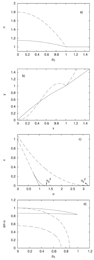
Figure 8 Parabolic refractive index profile. For a system characterized by a parabolic refractive, index we display: n as a function of ρ0 in panel a), y as a function of x in panel b), v as a function of u in panel c), and sin a as a function of ρ0 in panel d). Solid lines correspond to n0 = 1:15 and dashed lines correspond to n0 = 1:8, being n1 = 1 in both cases.
5.Looking for n(p) for a given confinement regions.
In this section, we deal with the reverse problem we have just addressed, namely: given a desired confinement region, to find the right n(p). Many aspects of the problem we intend to analyze have been approached experimentally. What we intend in this article is to carry out a theoretical study on the topic, reaching analytical or numerical solutions within the framework of the geometric optics we are working with.
For clarity, we will talk in this section in terms of the four planes we have been
working with. We call plane a), b), c), and d) (which correspond to panels a), b),
c), and d), respectively, in Figs. 3, 4, and 8 to
the planes (p,n), (x,y), (u,v), and
In the previous sections, for every n(p) taken as an example, we have been able to
move from the plane a) to plane d), through planes b) and c), without any
complication. For the sake of analyzing the possibility of performing the reverse
way, we might think that we could move from plane d) to plane c) because of Eqs. (8)
and (9), which link 𝑢 and 𝑣 with
and
Finally, since
Unfortunately, it is not possible to move from
It is needful to remember that, for one step-index waveguide, for example, u and v are always
related by Eq. (6) or Eq. (7) on the curves that limit the zone containing the slope
and intercept values of straight lines that cut y(x) twice. In the same way,
What we have expressed in the previous paragraph allows, with some restrictions, to
design a waveguide in
By means Eqs. (28), (30), (31), (32), and (33), which remain valid as long as n have
a parabolic radial variation, we have built Fig.
9, where n0 is represented as a function of
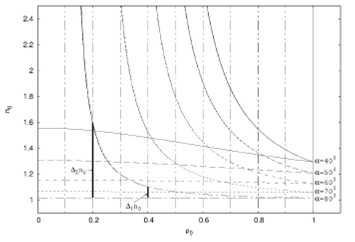
Figure 9 n0 as a function of ρ0 for different a values. For every a value, two curves are displayed, which enclose the feasible n0 and ρ0 combinations so that the radiation is confined.
The last expression has been obtained from Eqs. (28), (31), and (32) taking into
account that
Although Fig. 9 has been built for n1 = 1, it could be done for any n1 value by solving the corresponding equations iteratively.
From Fig. 9, it follows that, for a given angle
with which the radiation enters the guide, the farther from the axis it does, the
more precise the n0 value (for a given n1) with which the
guide should be constructed so that the radiation kept confined. This point is
illustrated with two examples included in the figure. Radiation entering the guide
making an angle with the axis of 10o, that is to say, α =80o,
at a distance
Then, in the figure, a design method consisting in choosing
Also, for one-step and multi-step refractive index profiles, clearly, an adequate
construction of the guide will allow wider margins in
In Fig. 10, where the confinement region for
the ith step is represented, two points,
and doing sinα = 0 in Eq. ([diente1]), we obtain

6.Summary and Conclusions
Based on the criterion we have set in PII applying the Fermat’s extremal principle in
the framework of the geometrical optics, in this article, we have depicted the
radiation confinement regions in the plane
If different types of the electromagnetic wave can propagate within the system, the angle and distance from the axis with which the radiation enters the guide, parameters defined according to the technological needs, require to be well differentiated. Choosing those parameters properly, the methodology allows us to define propagation modes through the different regions of the guide, and, in design processes, by building suitably the waveguide, the technique can be used as a resource to limit the parameters that characterize the system.

