


 nova página do texto(beta)
 Artigo em XML
 Referências do artigo
 Enviar este artigo por email
 Citado por SciELO
  Similares em
SciELO
Similares em
SciELO 
 Permalink
1. Introduction
In this paper we present a systematic comparison of various signal processing methodologies that perform matrix factor decompositions with an application to underlying systematic risk factors and betas driving returns on equities. The contribution of this study is to find the risk factors and betas in decompositions that are based on different hypotheses. These hypotheses are of statistical and linear algebra type, and allow to see the problem from different points of view. An interesting aspect is the possible extension of the approaches we present to different areas as multivariate asset pricing models, as methodologies based on different underlying assumptions provide different decompositions and explanations.
In previous studies, we tested different approaches to dimension reduction in the context of a statistical approach to the Arbitrage Pricing Theory (APT). The approaches were based on, the estimation of the underlying multifactor model driving the returns on equities of the Mexican Stock Exchange. The models consisted of different dimension reduction and feature extraction techniques under a statistical approach. Under this conceptualization, both the systematic risk factors and the sensitivities to those factors (betas) can be computed from the observed returns on equities. There are two differentiated stages, namely, the risk extraction and the risk attribution processes; the empirical studies have only focused on the former.
A methodology related to the contribution we make is that of intertemporal decomposition (see for example Collins & Kothari (1989) and Le & Miller (2004)), which seeks to explain changes in stock market values through simultaneous cross-sectional and temporal analysis. An important difference with our approach is that it includes an ARMA model for the temporal modelling, while in this publication we perform a matrix decomposition under different hypotheses, without seeking a temporal structure that includes memory in the ARMA style. The advantage of our approach is that it allows us to deal with time series with time-varying statistics, which is not possible with ARMA-type models that assume stationarity of the time series.
In this context, in a first study, Ladrón de Guevara & Torra (2014) estimated the underlying structure of systematic risk by using Principal Component Analysis (PCA) and Factor Analysis (FA)1; it included the testing of the models in two versions: returns and returns over the riskless interest rate for weekly and daily databases, and a two-stage methodology for the econometric contrast. First, they extracted the underlying systematic risk factors using both the standard linear version of Principal Component Analysis and the maximum likelihood Factor Analysis estimation, and they were able to reconstruct the observed returns using the factors extracted almost perfectly in all cases. Then, for all the systems of equations, they simultaneously estimated the sensitivities to the systematic risk factors (betas) by Weighted Least Squares (WLS). Finally, they tested the pricing model by using an average cross-section methodology via Ordinary Least Squares (OLS), corrected by a heteroskedasticity and autocorrelation consistent (HAC) estimation of covariances. Their results showed that the APT was highly sensitive to the extraction technique utilized and to the number of components or factors retained. This suggests that the model explains partially the variations in average returns on the selected stocks of the Mexican Market for the periods and the methodology considered.
In a second study, Ladrón de Guevara, Torra & Monte (2018) tried to make apparent a more realistic latent systematic risk factor structure utilizing the Independent Component Analysis2, to find out whether the model performed better on the Mexican Stock Exchange, using the systematic risk factors and betas extracted via this technique, which is more appropriate for parallel and non-Gaussian financial time series. To ensure the correct performance of ICA and to demonstrate that the extraction of betas by classic multivariate may not be very reliable, they first tested the univariate and multivariate non-Gaussianity of the data utilizing the Jarque-Bera test for univariate normality and the Mardia3 and Henze-Zirkler4 tests for multivariate normality. In addition, to homogenize the criteria of ranking in the four techniques, they sorted out the independent component extracted by using the criteria proposed by García-Ferrer et al. (2008). The estimation of the multifactor generative model of returns also reproduced the observed returns almost perfectly in all the cases. The evidence found in the econometric contrast showed mixed results for the acceptance of the APT.
In a third study, Ladrón de Guevara, Torra & Monte (2019) used the Nonlinear Principal Component Analysis5 (NLPCA) as an extension of the standard Principal Component Analysis (PCA) that overcomes the limitation of the PCA’s assumption about the linearity of the model. NLPCA belongs to the family of nonlinear versions of dimension reduction or underlying features extraction techniques, including nonlinear factor analysis and nonlinear independent component analysis, where the principal components are generalized from straight lines to curves. NLPCA can be achieved via an artificial neural network specification where the PCA classic model is generalized to a non-linear model, namely, Neural Networks Principal Component Analysis (NNPCA). The authors used an auto-associative multilayer perceptron neural network or autoencoder, where the ‘bottleneck’ layer represents the principal nonlinear components, or in this context, the scores of the underlying factors of systematic risk. This neural network represents a powerful technique capable of performing a nonlinear transformation of the observed variables into the principal nonlinear components and executing a nonlinear mapping that reproduces the original variables. The evidence found showed that the reproductions of the observed returns using the estimated components via NNPCA were almost perfect in all cases; nevertheless, the results in an econometric contrast led to a partial acceptance of the APT in the samples and periods studied.
Finally, in a fourth study Ladrón de Guevara, Torra & Monte (2021) made the first attempt to make a comprehensive comparison of the four aforementioned techniques. From the theoretical standpoint, and as a consequence of the financial data nature the estimated factors should be superior as we progress from classical techniques, i.e., Principal Component Analysis and Factor Analysis, to more sophisticated techniques, i.e., Independent Component Analysis and Neural Networks Principal Component Analysis; however, their internal assumptions, procedures, and algorithms, make the direct comparison among either the extracted factors or the factor loadings, produced by each one of them, impracticable. This fact led to compare the former techniques in such a way that they could be measured homogeneously. To present an objective and homogeneous comparative study concerning techniques, they carried on their research according to two different perspectives. First, they evaluated them from a theoretical and matrix scope, making parallelism among their particular mixing and demixing processes, as well as among the attributes of the systematic risk factors extracted by each method. Secondly, they carried out an empirical study to measure the level of accuracy in the reconstruction of the original variables, reproduced by the multifactor generative model of returns, when the underlying systematic risk factors estimated employing each extraction technique were employed. The results showed that the reproduction capacity of the four techniques was very good; being, NNPCA the one that presented the lowest level of error in reconstruction in almost all the cases and experiments, followed by PCA, FA, and ICA.
In this context, the objective of this research is to continue the comparative study across these four techniques from three additional perspectives and methodologies: 1) through a comparative statistical and graphical analyses of both, the underlying risk factors and their corresponding sensitivities (betas); 2) using the comparative analysis of the results obtained in the econometric contrast of the APT, when the systematic risk factors and betas computed in each technique are used; and 3) utilizing a comparative analysis about the interpretation of the extracted underlying systematic risk factors.
To the best of our knowledge, there are no comparative studies involving these four dimension reduction or feature extraction technique in literature, and much less in the Finance field, so in this sense, this fact represent one of the main contributions of this paper. In addition, the context where the empirical study is done represents an emerging financial market where this kind of study is scarce. Finally, the empirical findings of this research have potential applications in the hedging and risk management industry, since they identify and compare different underlying systematic risk factors estimated by four different and powerful statistical and computational extraction techniques, that may be useful for the banks and financial institutions in the portfolio management and asset allocation by mimicking and hedging the systematic risk factors extracted and identified by PCA, FA, ICA, and NNPCA, according to their needs and investment objectives.
The rest of this paper is structured as follows: in section 2 we present a review of literature; in section 3, we describe the methodology used in this research; in section 4, we present the results of the empirical study and propose a discussion related to our findings; and in section 5 we draw some conclusions and future lines of research. Finally, in section 6 we include the references consulted.
2. State of the art
As far as we concerned comparative studies involving the four techniques, i.e., PCA, FA, ICA, and NNPCA are inexistent in literature, except in the case of that performed by Ladrón de Guevara, et al. (2021). In that study authors make a review of the state of the art of studies that compare some of the aforementioned techniques in the field of Finance. Thus, with the purpose of not being redundant with the review of literature done in the foregoing study and to complement it, in this paper we only revisit a seminal reference on this issue and we update the review of literature on this matter. In this case, we include some relevant references of comparative studies of these techniques and we present some studies that mix some of them with applications in other fields of knowledge in addition to Finance. The nature of techniques such as ICA and NNPC made that their original use had been in sciences and disciplines such as Biochemistry, Astronomy, Neurosciences, Computer Sciences, Telecommunications, Signal Processing, Artificial Intelligence, Data-Mining, Encephalography, Voice and Images Recognition, etc.; however, by studying those applications one can detect their potential in other fields such as Finance and Economics.
The study of Scholz (2006) is the only one that we detect comparing three of the techniques used in this paper: PCA, ICA, and NNPCA, which make that study a seminal reference for comparative analysis in this kind of dimension reduction techniques. In his study, Scholz uses these three techniques in the context of biochemistry to extract biologically meaningful components from molecular data. That research reveals that there are benefits and drawbacks in each technique and that the suitability of one over the others will depend on the characteristics of data and the objective of the research.
Some other relevant and updated comparative or mixing studies involving PCA, FA, ICA, and NNPCA in different fields of knowledge are the following.
Firstly, Cunningham & Ghanramani (2015) present a survey of a great number of linear dimensionality reduction techniques where PCA, FA, and ICA are considered. In their study, they also make some generalization of all the techniques analyzed. Likewise, de Winter & Dodou (2016), present a comparison of the loadings estimated by PCA and FA through simulations finding different patterns in the estimations of each technique. Moreover, Han & Fyfe (2020) compare a set of methods for preprocessing time series data, where PCA, FA, ICA, and another technique named Complexity Pursuit (CP) are considered, to obtain underlying factors that subsequently will be used in a multi-layer perceptron with forecasting purposes. They found that FA and ICA had the worst performance.
In Biomedical Sciences, Uğuz (2012) combines PCA and artificial neural networks to extract, reduce and classify data related to the diagnosis of heart valve diseases.
In Medical Sciences, Yang, Si, Wang & Zhang (2020) develop ICA-PCA networks to extract electrocardiogram features. Likewise, Rabbi, Pizzolato, Lloyd, Carty, Devaprakash, & Diamond (2020), compare Non-Negative Matrix Factorization (NNMF) with PCA, FA, and ICA, to determine the best method for extracting muscle synergies in dynamics tasks, such as walking and running.
In the field of Signal Processing, You & Hung (2021) use PCA, FA, and ICA in the context of dimensionality reduction of spectral-temporal video and audio signals, finding that ICA and FA obtained features with higher identification accuracy.
In Agrosciences and Physics, Zhou, Huang, Fan, Zhao & Liang (2020) compared the results of another novel extraction technique (Support Vector Machine (SVM) based on Competitive Adaptive Reweighted Samplings (CARS)) with those of a set of dimension reduction techniques where PCA, FA, and ICA were included. This research was developed in the context of the classification of varieties of sweet maize seeds based on hyperspectral images.
In Geophysics, Li, et al. (2019), compare PCA and ICA in the context of regional crustal displacement in the Antarctic, finding that ICA was better than PCA regarding the accuracy of the Global Navigation Satellite System (GNSS).
In Telecommunication Sciences, PCA, FA, and ICA were also compared with another novel technique called Kernel Entropy Component Analysis. In their study, Berruet, Baala, Caminada & Guillet (2020), applied all these techniques to evaluate the suitability for the implementation of future fingerprinting solutions for indoor localization.
In Computer Sciences, Arslan, Akyürek & Kaya (2017) compare the performance of classification methods for hyperspectral image data using dimensional reduction techniques. Among the techniques used in their research, they include PCA and ICA. Their results show that the dimension reduction utilized may have significant effects on classification performance.
In Urbanistic and Environmental Studies, Gielen, Riutort-Mayol, Palencia-Jimenez & Cantarino (2018) compare PCA, FA, ICA, and Bayesian Factor Analysis (BFA) to analyze the phenomenon of urban sprawl at the municipality level in Valencia, Spain.
Finally, in the field of Finance, other relevant studies that combine two of the techniques studied in this paper are the following. On one hand, Juanwei, Shenggang & Jimin (2017), combinate PCA and ICA, and also Variational Mode Decomposition (VMD), to determine the components that explain the gold price. On the other hand, Liu & Wang (2011), propose some models to predict the Chinese Stock Market, where they use PCA and ICA to obtain the latent components, which later are used as inputs of a Back Propagation Neural Network (BPNN). Their results showed a better performance of the models that integrated the pervasive components extracted by ICA. Additionally, Lassan & Vrins (2021), compare the performance of PCA and ICA in optimization of large investment universe portfolios, finding that ICA produces better dimensionality reduction estimations that lead to the superior risk-adjusted performance of investment portfolios.
3. Methodology
To understand the motivation of the comparison methodology proposed in this paper, below is a summary of the extraction processes of each one of the techniques used in this work, which are presented next.
Principal Component Analysis6
Where: Z = Matrix of principal components, X = Matrix of data, A = Matrix of loadings.
Factor Analysis7
(Bartlett’s model)
Where: F = Matrix of common factors, X = Matrix of data, Λ = Matrix of loadings, ψ = Matrix of specific variances or matrix of specificities or uniqueness, µ = Vector of means.
Independent Component Analysis8
Where: S = Matrix of independent components or original sources, X = Matrix of data, W = Demixing matrix.
Neural Networks Principal Component Analysis9
Where: Z = Matrix of nonlinear principal components, X = Matrix of data, W1 = Matrix of weights from the first layer to the second layer, W2 = Matrix of weights from the second layer to the third layer, g = Transferring non-linear function.
Thus, from an interpretation standpoint of the extracted factors, we could say that for PCA, FA and ICA, these factors may be interpreted as the coordinates of the observations in the space spanned by the demixing matrix of their extraction processes. That is, first in PCA, the matrix A may be interpreted as a projection operator with directions that correspond to the least error reconstruction. Secondly, in FA the matrix C may be interpreted as an operator that generates the variation around the mean value of the observations. Finally, in ICA the matrix W, represents a matrix that mixes unobservable factors using the criterion that the observable ones will have a maximum non-Gaussian distribution. On the other hand, although in NNPCA, we do not have a single demixing matrix, we could interpret the two matrices involved in the demixing process. That is, matrix W1 may be interpreted as the parameters of an operator that makes a non-linear transformation of data (i.e. a matrix followed by a vector nonlinearity), which makes the function of the first layer of the network to be different from that of the other methods; while matrix W2 makes a dimensionality change of the representation given the output of the first layer.
In other words, considering that the matrices that generate the observations are obtained by way of different criteria and they look for finding different representation of data, these matrices result not easily comparable in the sense that we are trying to compare objects with different dimensions. As an analogy, it is as if we would like to compare time and space units of measurement.
Consequently, in this paper we propose a comparative approach focused on three different fields where the results of each one of the four extraction techniques can be compared: 1) an statistical and graphical analysis of the elements of the underlying systematic risk structure, 2) the results of the econometric contrast of the APT model that used the underlying risk factors extracted and 3) the interpretation given to those pervasive factors.
The empirical data and a description of the techniques and procedures used in each kind of comparison method are explained in the next sub-sections.
3.1 The data
The data used in the empirical comparative study is derived from the results of our previous studies focused on each one of the analyzed dimension reduction techniques. Thus, for the sake of the comparative approach of this paper, we keep the same databases. This data corresponds to stocks of the Price and Quotation Index (IPC) of the Mexican Stock Exchange (BMV). Both the period analyzed and the shares selected reflect the availability of data among the diverse information sources consulted and our purpose to test these techniques in a normal period before the last confirmed financial crisis: the subprime crisis.
Our basic aim, since our particular work dedicated to each technique, was to build a homogeneous and sufficiently broad database, capable of being processed with the feature extraction techniques used in this study in the normal period before the crisis subprime. In addition, although the four techniques used in our studies involve both explanatory and forecasting potential, in this first stage of our researches we have centered our efforts on the explanatory power, so that, we can test the forecasting power in future researches in the next adjacent period ranging from the date after the period of these studies to the date before the bursting of the speculative bubble originated by the subprime financial crisis.
In this context, we have worked with four different databases to test different expressions and periodicities of the returns on equities. On one hand, two databases are expressed in returns and the other two, in returns in excesses of the riskless interest rate. On the other hand, two of them have weekly periodicity and the other two a daily one.10
3.2 Underlying systematic risk structure: Statistical and graphical analysis.
To continue the comparative study across the four techniques, we propose an analysis by way of 1) a descriptive statistical analysis and 2) graphical or morphological analyses considering the elements of the underlying systematic risk as signals.
On the other hand, the APT is integrated by two main assumptions, the generative multifactor model of returns and the arbitrage absence principle or arbitrage principle; however, our study has been focused only on the first part, i.e., the improved estimation of the generative multifactor model of returns under a statistical approach. Consequently, we consider that a deeper analysis of the estimated underlying systematic risk structure estimated by each technique may represent a suitable manner to compare the results obtained in each technique.
In the four techniques used in our work, we estimated that underlying structure of systematic risk, whose risk factors (Fs) and sensitivities to them (β) will be compared under the aforementioned perspectives. Following the comparative spirit of this paper, we respect the specifications of the window test used in the particular studies devoted to each technique, which ranged from two to nine extracted factors in each technique and each database. The foregoing criteria included: the eigenvalues arithmetic mean, the explained variance, the exclusion of factor with a small power of explanation, the scree plot, the Q statistic, the likelihood ratio contrast, the AIC, the BIC, and the maximum number of extracted components.11
Therefore, we will compare the four techniques using the statistical and graphical analyses of both, the underlying risk factors and their corresponding sensitivities (betas) estimated in our experiments.
3.3 Econometric contrast of the Arbitrage Pricing Theory (APT).
Following the methodology used in previous studies, we employed the extracted risk factor by each technique in the context of a statistical approach to the APT which consider that the nature and number of risk factors pricing the returns on equities can be estimated by some statistical and computational techniques capable to extract those factors from the stock's historical prices.
Following Ross (1976) the APT assumes the following generative multifactor model of returns:
Where, ( ji represents the sensitivity of equity i to factor j, F jt the value of the systematic risk factor j in time t common for all the stocks, and ( i the idiosyncratic risk affecting only equity i.
In the four techniques used in our studies, we estimated this underlying structure of systematic risk, whose risk factors (Fs) and sensitivities to them (β) will be compared in this paper. To perform the econometric contrast of the underlying structure of systematic risk, under the framework of the statistical approach to the APT, in our previous studies we have followed a two-stage methodology.
In the first stage, we took the estimated underlying factors or scores of each technique and regressed them in the logarithmic returns on equities of our sample, to compute a simultaneous estimation of the sensitivities or betas of the entire system of equations. We adopted this methodology because it solves the classic econometric problems of autocorrelation and heteroskedasticity across the residuals that a non-simultaneous estimation of the betas would imply.12 Due to the nature of our data and the mathematic algorithms utilized in each technique, we had to use two different methodologies for running this stage concerning the simultaneous computation of the betas. For PCA, FA and ICA, we used the Weighted Least Squares (WLS); and for NNPCA, we used the Seemingly Unrelated Regression (SUR).
The WLS methodology or cross-equation weighing accounts for cross-equation heteroskedasticity by minimizing the weighted sum-of-squared residuals. The equation weights are the inverses of the estimated equation variances and are derived from the unweighted estimation of the parameters of the system. This method yields identical results to unweighted single-equation least-squares if there are no cross-equation restrictions.13
The SUR methodology also known as the multivariate regression, or Zellner's method, estimates the parameters of the system, thus accounting for heteroskedasticity and the contemporaneous correlation in the errors across equations. The estimates of the cross-equation covariance matrix are based upon parameter estimates of the unweighted system.14 The SUR methodology supplies better estimators than WLS in the system of equation computing of parameters, free of the autocorrelation and heteroskedasticity in the residuals of the model, which estimates the betas more reliable.
In the second stage, we use the betas estimated in the first step as regressors of a cross-section model to explain the average returns on equities of our sample, following the classic methodology for testing the APT. Following Amenc and Le Sourd (2003) the APT fundamental pricing equation:
posits that betas are the sensitivities to the systematic risk factors and that lambdas are the risk premium paid by the market for being exposed to each class of systematic risk. Subsequently, this pricing equation can be tested utilizing an average cross-section methodology:
In our previous studies, we computed the coefficients of the model by using ordinary least squares (OLS) and correcting the estimated standard errors employing the Newey-West heteroskedasticity and autocorrelation consistent estimates of covariances (HAC).15 Additionally, we verified normality in the residuals by carrying out the Jarque-Bera test of normality.
According to Gómez-Bezares (2000), the APT pricing model requires the statistical significance of at least one lambda parameter different from λ0,16 and the equality of the independent term to its theoretic value, i.e., the average returns, in the models expressed in returns:
and zero, in the models expressed in excesses of the riskless interest rate:
In our previous studies, we used the Wald test to confirm these equalities.
In addition, to be very strict in the acceptance of the estimated models we have considered a criterion where we only accepted the models where not only the two previous requirements were fulfilled, but also when the results of the regression warranted a high adjusted R 2 , a global statistical significance of the model given by the F statistic, and also fulfilled normality in the residuals of the estimation measured by the Jarque-Bera test.17
3.4 Interpretation of the underlying risk factors.
Finally, to compare whether the meanings of each risk factor, in the four databases, maybe similar across the four techniques, in this section we will compare the interpretation given to the extracted factors across techniques, under the scope of the interpretation methodology used in Ladrón de Guevara & Torra (2014), which considers the sector interpretation approach based on the factor loadings matrices of the extraction process in each technique. This approach relates the loadings of each stock in each extracted factor with a sector or combination of sectors, to give an interpretation or name to each factor, derived from the stocks that contribute to the formation of each systematic risk factor.
In this context we propose two techniques to perform the aforementioned comparison: 1) a graphical analysis of the loading matrices and the extracted factors, to inspect visually the contributions, weights, and signs of each stock or group of stocks to each risk factor, and 2) a set of comparative tables that confront the interpretation given to each extracted factor across the four techniques.
4. Results and discussion
4.1 Underlying systematic risk structure: Statistical and graphical analysis.
This section presents the results of the comparative study of both the underlying systematic risk factors extracted by PCA, FA, ICA, and NNPCA, and the sensitivities to them (betas) estimated in the extraction processes estimated in each of them for all our experiments. For the sake of saving space, we only present the results regarding the first factor estimated by each technique for the experiment when we extracted nine factors in the database of weekly returns; however, the conclusions derived from this analysis are similar for all the cases. Table 1 shows the descriptive statistics of the aforementioned factors18. Although the scores of the underlying factors in all the techniques are not normalized, the mean of them in all the techniques is almost zero. The standard deviation of all the extracted factors within each technique is very similar; however, it is quite different across techniques. The skewness and kurtosis coefficients as well as the Jarque-Bera test indicate that in almost all the cases, the underlying systematic risk factors are not univariate normally distributed.
Table 1 Descriptive Statistics. First underlying systematic risk factors extracted by PCA, FA, ICA, and NNPCA. Database of weekly returns. Nine components were estimated.
| PC1 | F1 | IC1 | NNPC1 | |
|---|---|---|---|---|
| Mean | -0.011147 | 0.043786 | -0.011864 | 0.008312 |
| Median | -0.025207 | 0.058395 | -0.008407 | -0.008041 |
| Maximum | 0.622778 | 3.271584 | 0.431340 | 0.734043 |
| Minimum | -0.375429 | -3.465415 | -0.538880 | -0.398930 |
| Std. Dev. | 0.128976 | 1.001470 | 0.116841 | 0.142438 |
| Skewness | 0.921649 | -0.266661 | -0.284181 | 0.972586 |
| Kurtosis | 5.568533 | 4.412059 | 5.186298 | 5.869496 |
| Jarque-Bera | 121.1907 | 27.62492 | 61.87307 | 145.7147 |
| Probability | 0.000000 | 0.000001 | 0.000000 | 0.000000 |
| Observations | 291 | 291 | 291 | 291 |
Source: Own elaboration.
As expected, given the theoretical construction of the four techniques, the underlying factors are uncorrelated with each other in almost all the cases in the four databases, as the corresponding correlation matrices show19. In most of the cases, the correlation was zero and we couldn’t reject the null hypothesis of non-correlation at a 5% of statistical significance, except in the case of the ninth non-linear component extracted using NNPCA in the four databases, where we reject the null hypothesis of non-correlation; nevertheless, the correlation value of this component with the rest of them was negligible20.
Therefore, in the light of the foregoing analysis, we may state that from a statistical descriptive scope, the extracted factors via the four techniques have similar behavior. Next, we will analyze if the shape of them is similar, to detect if the factors extracted by way of the four techniques may be similar from a morphological standpoint.
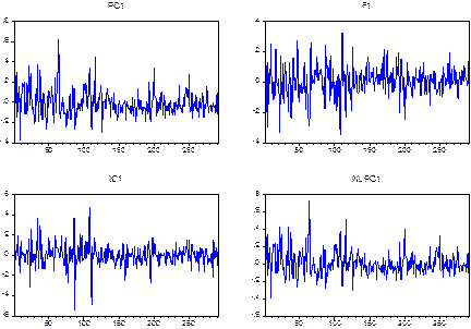
To visually analyze the systematic risk factors estimated by each technique, we construct individual plots to compare the shape of each systematic risk factor extracted by each technique respecting the ranking produced by each one of them, which satisfies the criteria of the amount of variability explained. It is important to remark that this experiment represents only a first approach to detect whether the factors extracted by each technique might be the same or similar across techniques. For the sake of saving space, in Figure 1 we only present the plots of the first risk factor extracted by each technique in the databases of weekly returns.21 As we can observe the factors estimated by PCA and NNPCA are very similar, which leads us to think that they could be almost the same systematic risk factors from a morphological standpoint. On the other hand, factors computed by FA and ICA in some periods of the observations present some similarities as well, but not at the same level as NNPCA and PCA, in points of high volatility, they behave quite differently. In addition, the volatility observed in the factors produced by FA and ICA is very high compared with that presented in PCA and NNPCA components. Finally, the values of the extracted factor by each technique vary as well; FA and ICA present higher values than those produced by PCA and NNPCA.
Source: Own elaboration.
Figure 1 First underlying systematic risk factor extracted by the four techniques. Multiple graphs. Database of weekly returns. Nine factors estimated.
On the other hand, we made the same analysis of the matrix of sensitivities to the underlying systematic risk factors or betas, whose results are presented following the same structure of those corresponding to the risk factors. First, in line with the previously reported in this paper, Table 2 shows the descriptive statistics regarding the first beta computed in each technique for the experiment when we extracted nine factors in the database of weekly returns; however, the conclusions derived from this analysis are similar for all cases22.
Table 2 Descriptive Statistics. Descriptive Statistics. Matrix of Betas computed by PCA, FA, ICA, and NNPCA. Database of weekly returns. Nine components estimated.
| B1-PCA | B1-FA | B1-ICA | B1-NNPCA | |
|---|---|---|---|---|
| Mean | -0.213564 | -0.113065 | -0.113065 | -0.541890 |
| Median | -0.213982 | -0.140755 | -0.140755 | -0.557320 |
| Maximum | -0.097420 | 0.031415 | 0.031415 | 5.139106 |
| Minimum | -0.328798 | -0.243882 | -0.243882 | -3.890342 |
| Std. Dev. | 0.067983 | 0.084422 | 0.084422 | 2.098866 |
| Skewness | 0.028040 | 0.196405 | 0.196405 | 0.718213 |
| Kurtosis | 2.000887 | 1.749982 | 1.749982 | 3.900535 |
| Jarque-Bera | 0.834476 | 1.430704 | 1.430704 | 2.395237 |
| Probability | 0.658864 | 0.489020 | 0.489020 | 0.301912 |
| Observations | 20 | 20 | 20 | 20 |
Source: Own elaboration.
One of the main findings is that the mean of the values of the betas, in general, is very small, as they are practically zero in all cases, except in the case of the beta number nine extracted via NNPCA in the database of weekly returns, which presents very higher values concerning all other cases. This beta reached a mean value of 3.642261, while the second larger absolute values ranged around 0.21 (PC1 in DBWR) and 0.54 (NNPC1 in DBWR); in general, the average higher values of the betas were produced by NNPCA. Another remarkable point is that in many cases the average sensitivities to some underlying systematic risk factors are negative, as in the case of the sensitivity to the first, fourth, and sixth principal components; to the seventh factor of FA; to the first, second, sixth, seventh and ninth independent components; and the first, seventh and eight principal nonlinear components. Under a financial interpretation, the negative sensitivities imply that the reaction of the returns to the variation of those betas would be inversely proportional. Moreover, changes in the returns on equities about change in the value of these betas, would be very small in the most cases.
The standard deviation of the betas is very similar within the factors extracted by each technique but quite different across them. In most cases, the skewness and kurtosis produce values closer to those corresponding to a normal univariate distribution, which is confirmed by the Jarque-Bera test, except in nine cases spread in PCA, FA, and NNPCA. The correlation matrices show that the betas are uncorrelated as well, except in some cases of the betas estimated in NNPCA23.
Therefore, in line with the foregoing analysis, we may state that from a statistical descriptive standpoint, the estimated betas related to the underlying risk factors by PCA, FA, and ICA present a similar behavior; however, those computed in NNPCA differs significantly from the former ones.
Next, we will analyze the shape of the sensitivities to factors, to detect if the betas computed for the four techniques could be similar from a morphological standpoint.
To visually analyze the betas estimated by each technique we also plot the individual betas of each factor to compare their shape and detect whether or not they were similar across the four techniques. The sensitivities to the first factor in the databases of weekly returns when nine factors were computed are presented in Figure 2.24 In general, the betas are different in the four techniques; nevertheless, in some points the betas estimated for PCA, FA and ICA present similar shapes but NNPCA behaves differently. Moreover, the volatility observed in the betas from the first two techniques shows a higher level than that produced by these last two techniques. As we have detected in the descriptive analysis, the highest values of the betas correspond to NNPCA, while the lowest corresponding to FA. In addition, the former present the highest variability, and the latter the lowest. Consequently, these results revealed that the sensitives to the underlying risk factors extracted by way of PCA, FA, ICA, and NNPCA are different and change significantly for each stock studied.

4.2 Results in the econometric contrast of the APT.
The objective of this section is to compare the results of the econometric contrast of the APT across the four techniques when the systematic risk factors and betas computed in each technique were used as inputs in the APT pricing equation.
This study has been focused on the improved estimation of the generative multifactor model of returns under a statistical approach of the APT. Nevertheless, we recognize that some of the results obtained in the econometric contrast may have been originated due to problems in the another part of this pricing model (the arbitrage principle); consequently, the results in the econometric contrast should be seen under this light. Future lines of research will be focused on this aspect of the model.
For the sake of saving space, we will not present in this paper the results in the econometric contrast obtained in each technique; however, the interested reader can consult the details in the previous research that correspond to each technique.25 In this paper, we intend to compare the main results in the econometric contrast across the four techniques.
Table 3 presents the models that fulfill all the requirements in the econometric contrast of the APT, according to the criteria established in section 3.3. PCA and FA were the techniques that produced the smallest number of models that fulfilled all the requirements in only three models. ICA and NNPCA were the techniques that generated the biggest number of them, with four. Interestingly, only the models expressed in returns produced completely accepted validation of the APT. In general, the models accepted in each technique were different; nevertheless, some models were accepted in two and three techniques. Those models were: the one with six and eight factors that were accepted in both ICA and NNPCA, and with seven in PCA and NNPCA, in the database of weekly returns. Regarding the database of daily returns, those models were the ones with three factors that were accepted in PCA, ICA, and NNPCA; and with nine, in PCA and FA. These findings may indicate some relevance of these specifications; however, a deeper analysis will be necessary on this matter.
Table 3 Models that fulfill all the requirements in the econometric contrast of the APT.
| PCA | FA | ICA | NNPCA | |
|---|---|---|---|---|
| Database of weekly returns. | ||||
| Model witd 5 betas | ○ | |||
| Model witd 6 betas | ○ | ○ | ||
| Model witd 7 betas | ○ | ○ | ||
| Model witd 8 betas | ○ | ○ | ||
| Database of daily returns. | ||||
| Model witd 3 betas | ○ | ○ | ○ | |
| Model witd 5 betas | ○ | |||
| Model witd 8 betas | ○ | |||
| Model witd 9 betas | ○ | ○ | ||
Notes: PCA: Principal Component Analysis; FA: Factor Analysis; ICA: Independent Component Analysis; NNPCA: Neural Networks Principal Component Analysis; ○= Model which fulfills all the requirements of the econometric contrast.
Source: Own elaboration.
Although only the models presented in Table 3 were the ones that fulfilled all the requirements of the econometric contrast of the APT, there were some other specifications of the model where we found partial evidence supporting the multifactor structure of the underlying systematic risks; i.e., models where betas different from β 0 were statistically significant but where β 0 was not equal to its theoretic value. To compare these results across techniques, in Table 4 we show the value of the estimated lambdas (risk premiums) corresponding to the betas that were statistically significant in all the models. Models considering only two factors obtained the worst results; the rest of the specifications showed a relatively similar performance considering the number of statistically significant factors. The sensitivity to the underlying systematic risk factor that was statistically significant in most of the models was the β 3 followed by β 2 , and then by β 5 and β 6 , which may point to them as interesting factors to be analyzed more deeply.
Moreover, the general values of the risk premiums produced in all models and across the four techniques are really low, in all the cases they produced values smaller than one; additionally, many of them presented a negative sign. Finally, we made an additional statistical analysis of the estimated risk premiums, where we could detect the following interesting findings:26
FA detects 38% of the total statistically significant risk premiums, but its values are those with the greatest dispersion in the weekly databases. Conversely, for daily data FA only contributes with 28% of the relevant risk premiums at the same level that ICA; which could be explained because the higher moments of daily data are more relevant than those related to weekly data since in the latter there is less noise. In addition, there is a higher dispersion in the FA values than in the other techniques as well.
Regarding the behavior of the relevant risk premiums in the function of the dimension of the model to contrast (number of betas), we observe that for the weekly databases, the higher the dimension of the model, the greater the grade of outliers in the risk premiums values; which becomes the models with the highest number of betas (8 and 9) those with the greatest dispersion of their values. In opposition, the dispersion in the daily does not change depending on the dimension, and it is not so evident the increase of atypical risk premiums as the number of betas considered in the model grows. If we make a segmentation among techniques, FA always presents the major variability in the relevant risk premiums.
Concerning the ranking of the lambdas associated with the systematic risk factors, we can see that in both, the weekly and daily frequencies, FA and ICA reveal a bigger number of relevant latent factors than PCA and NNPCA.
Table 4 Betas statistically significant.
| DATABASE OF WEEKLY RETURNS | DATABASE OF WEEKLY EXCESSES | DATABASE OF DAILY RETURNS | DATABASE OF DAILY EXCESSES | ||||||||||||||||||
|---|---|---|---|---|---|---|---|---|---|---|---|---|---|---|---|---|---|---|---|---|---|
| PCA | FA | ICA | NNPCA | PCA | FA | ICA | NNPCA | PCA | FA | ICA | NNPCA | PCA | FA | ICA | NNPCA | Total | |||||
| Model witd 2 betas | λ1 | λ1 | λ1 | λ1 | 0 | ||||||||||||||||
| λ2 | λ2 | λ2 | -0.00049 | -0.04908 | λ2 | -0.00052 | -0.04878 | 0.00046 | 5 | ||||||||||||
| Model witd 3 betas | λ1 | λ1 | λ1 | -0.03853 | λ1 | 1 | |||||||||||||||
| λ2 | 0.00296 | 0.01034 | λ2 | 0.00298 | -0.00195 | λ2 | -0.00057 | 0.02121 | -0.00302 | 0.00113 | λ2 | -0.00061 | 0.00085 | 10 | |||||||
| λ3 | -0.00770 | 0.12722 | 0.01665 | 0.02173 | λ3 | -0.00769 | 0.12758 | 0.01662 | -0.02129 | λ3 | -0.00137 | 0.01201 | -0.00104 | λ3 | -0.00141 | 0.00318 | 0.00162 | 14 | |||
| Model witd 4 betas | λ1 | λ1 | λ1 | 0.00113 | λ1 | 1 | |||||||||||||||
| λ2 | 0.00292 | -0.01492 | 0.00193 | λ2 | 0.00294 | -0.05436 | -0.01774 | -0.00237 | λ2 | 0.02701 | 0.00286 | 0.00090 | λ2 | -0.00043 | 11 | ||||||
| λ3 | -0.00777 | -0.01220 | 0.01002 | λ3 | -0.00776 | -0.00193 | 0.00891 | -0.00481 | λ3 | -0.00129 | 0.05664 | -0.00262 | -0.00184 | λ3 | -0.00132 | 0.00245 | -0.00140 | 14 | |||
| λ4 | 0.13780 | λ4 | 0.02853 | λ4 | 0.06924 | λ4 | 3 | ||||||||||||||
| Model witd 5 betas | λ1 | -0.07078 | λ1 | -0.07021 | λ1 | λ1 | 2 | ||||||||||||||
| λ2 | 0.00300 | -0.01771 | -0.00892 | λ2 | 0.00303 | -0.00505 | λ2 | λ2 | -0.00289 | -0.00080 | 7 | ||||||||||
| λ3 | -0.00762 | 0.02423 | λ3 | -0.00761 | -0.03206 | λ3 | -0.00130 | -0.00254 | -0.00229 | λ3 | -0.00133 | -0.00174 | 9 | ||||||||
| λ4 | λ4 | λ4 | 0.10101 | λ4 | 0.10455 | 2 | |||||||||||||||
| λ5 | 0.21077 | 0.00348 | λ5 | 0.20969 | λ5 | λ5 | 3 | ||||||||||||||
| Model witd 6 betas | λ1 | -0.09734 | λ1 | -0.09697 | λ1 | λ1 | 3 | ||||||||||||||
| λ2 | 0.00292 | -0.01899 | 0.00378 | λ2 | 0.00295 | -0.00404 | λ2 | λ2 | 6 | ||||||||||||
| λ3 | -0.00775 | -0.00997 | λ3 | -0.00775 | -0.00882 | λ3 | -0.00130 | 0.00401 | λ3 | -0.00133 | 0.00402 | 8 | |||||||||
| λ4 | λ4 | λ4 | λ4 | 0.00309 | 2 | ||||||||||||||||
| λ5 | 0.20782 | λ5 | 0.20709 | 0.00147 | λ5 | 0.00291 | λ5 | 5 | |||||||||||||
| λ6 | -0.13978 | λ6 | 0.01717 | λ6 | 0.05257 | -0.00162 | λ6 | 5 | |||||||||||||
| Model witd 7 betas | λ1 | λ1 | λ1 | -0.05676 | λ1 | -0.05971 | 2 | ||||||||||||||
| λ2 | 0.00292 | 0.02036 | 0.00362 | λ2 | 0.00294 | 0.00218 | λ2 | λ2 | 0.00222 | 6 | |||||||||||
| λ3 | -0.00776 | -0.01168 | λ3 | -0.00776 | -0.00650 | λ3 | -0.00130 | 0.00211 | λ3 | -0.00130 | 0.00146 | 8 | |||||||||
| λ4 | -0.15198 | λ4 | -0.15182 | λ4 | -0.12533 | 0.00288 | λ4 | -0.13575 | 5 | ||||||||||||
| λ5 | -0.06563 | λ5 | -0.06446 | 0.00168 | λ5 | 0.07379 | λ5 | -0.00065 | 5 | ||||||||||||
| λ6 | 0.07245 | λ6 | 0.00322 | 0.01431 | λ6 | 0.00119 | λ6 | 0.06580 | -0.00287 | 6 | |||||||||||
| λ7 | λ7 | -0.00500 | λ7 | 0.05998 | λ7 | 0.07526 | 3 | ||||||||||||||
| Model witd 8 betas | λ1 | -0.10643 | λ1 | -0.10598 | λ1 | 0.00244 | λ1 | -0.05614 | -0.00197 | 5 | |||||||||||
| λ2 | 0.00288 | -0.05528 | 0.01043 | 0.00303 | λ2 | 0.00290 | -0.05599 | 0.00439 | λ2 | 0.00329 | λ2 | 8 | |||||||||
| λ3 | -0.00783 | -0.06844 | -0.01765 | -0.02117 | λ3 | -0.00782 | -0.06776 | -0.02272 | λ3 | -0.00131 | -0.00163 | λ3 | -0.00134 | -0.00284 | 11 | ||||||
| λ4 | 0.12686 | λ4 | 0.12691 | λ4 | 0.00281 | λ4 | 0.06366 | 0.00096 | 5 | ||||||||||||
| λ5 | -0.08073 | λ5 | -0.08090 | λ5 | 0.05464 | λ5 | -0.00069 | 4 | |||||||||||||
| λ6 | 0.09068 | λ6 | 0.08932 | λ6 | -0.14354 | λ6 | -0.14532 | 0.00283 | 5 | ||||||||||||
| λ7 | 0.07573 | λ7 | 0.07557 | λ7 | λ7 | 0.03899 | 0.00028 | 4 | |||||||||||||
| λ8 | 0.17361 | λ8 | 0.17512 | -0.01046 | λ8 | 0.00267 | λ8 | 4 | |||||||||||||
| Model witd 9 betas | λ1 | -0.14932 | λ1 | -0.14882 | λ1 | λ1 | 0.00300 | 3 | |||||||||||||
| λ2 | 0.00290 | λ2 | 0.00292 | -0.01257 | 0.00613 | λ2 | -0.00050 | λ2 | -0.00052 | -0.00183 | 0.00281 | 8 | |||||||||
| λ3 | -0.00780 | 0.02016 | λ3 | -0.00780 | 0.04280 | -0.02391 | λ3 | -0.00136 | -0.00353 | -0.00361 | λ3 | -0.00139 | 0.00250 | 10 | |||||||
| λ4 | 0.05005 | λ4 | 0.04998 | λ4 | -0.00051 | -0.10860 | λ4 | -0.00055 | -0.10328 | 6 | |||||||||||
| λ5 | -0.01158 | λ5 | 0.01050 | λ5 | 0.00041 | 0.00288 | λ5 | 0.00041 | -0.00076 | 6 | |||||||||||
| λ6 | 0.16900 | λ6 | 0.16767 | λ6 | 0.00058 | λ6 | 3 | ||||||||||||||
| λ7 | 0.09160 | λ7 | 0.09366 | 0.01247 | λ7 | λ7 | 0.09296 | 4 | |||||||||||||
| λ8 | -0.11678 | λ8 | -0.11721 | -0.01057 | λ8 | λ8 | -0.07264 | 0.00274 | 5 | ||||||||||||
| λ9 | 0.10175 | λ9 | 0.10273 | 0.00941 | -0.00040 | λ9 | -0.00094 | 0.10590 | 0.00100 | λ9 | 0.00097 | 0.00109 | 9 | ||||||||
| Notes: PCA: Principal Component Analysis. FA: Factor Analysis. ICA: Independent Component Analysis. NNPCA: Neural Networks Principal Component Analysis. Numbers represent tde risk premium of betas tdat were statistically significant at 5 % of error. Total: Number of times tdat tde betas were statistically significant. | |||||||||||||||||||||
4.3 Interpretation of the underlying risk factors.
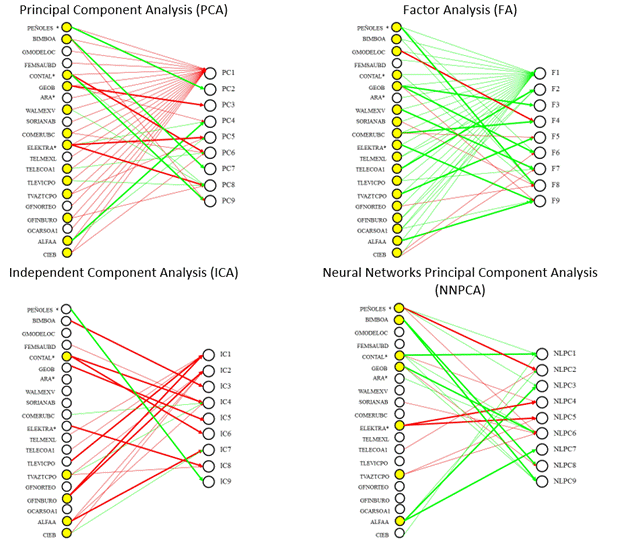
Figure 3 presents a schematic representation of the loading matrices that were used for the interpretation under an economic sector approach; i.e., the contribution of each stock in the formation of each extracted factor. This figure displays in green lines the positive loadings, and in red lines the negative ones. The wider the line the greater the contribution of each stock in the related factor. Circles next to the stock name filled in yellow color point the stocks with the higher frequency of contributions to different factors in each database. In line with the reported results, in this paper, we only present the figures that correspond to the experiment where nine factors were extracted in the database of weekly returns27.
As expected in theory, in PCA and FA we clearly can identify the first component or factor to the market one; however, in ICA and NNPCA we cannot do the same. Making a particular analysis by the database we can state the following.
In the database of weekly returns, when we use PCA, the stocks with the highest loadings in the components to which they contribute were: PEÑOLES*, BIMBOA, CONTAL*, GEOB, ELEKTRA* and ALFAA. On the other hand, the previous stocks are those with the highest frequency in their contribution to the formation of factors in addition to WALMEXV, COMERUBC, TELECOA1, TELEVICPO, TVAZTCPO, GFINBURO, and CIEB. Concerning FA, the highest loadings corresponded to PEÑOLES*, GMODELOC, GEOB, WALMEXV, COMERUBC, ELEKTRA*, TELECOA1, TVAZTCPO, and ALFAA; while all the stocks except FEMSAUBD and ARA* contributed in two or more factors. Concerning ICA, the highest loadings corresponded to PEÑOLES*, BIMBOA, CONTAL*, GEOB, ELEKTRA*, TELEVICPO, GFINBURO, and ALFAA; while the highest frequency was related to CONTAL*, TVAZTECPO, GFINBURO, ALFAA, and CIEB. Finally, in NNPCA the highest loadings were related to PEÑOLES*, BIMBOA, CONTAL*, GEOB, ELEKTRA*, and ALFAA; while the highest frequency matches with the previous stocks plus TVAZTECPO.
Additionally, we present a set of comparative tables about the interpretation of each ranked factor extracted by PCA, FA, ICA, and NNPCA for the database of weekly returns. Tables 6 presents the results regarding the experiment when nine factors were extracted, however we comment some relevant results derived from the analysis of the four databases when nine factors were extracted.28
Source: Own elaboration.
Figure 3 Loadings matrices. Diagram for interpretation of extracted factors for PCA, FA, ICA, and NNPCA. Database of weekly returns. Nine components.
In general, the interpretation of the same factor across the four techniques is not constant, except in the case of the market factor identified with factor number one for PCA, FA, and ICA, in the database of daily excesses. In addition, the market factor was identified in the four databases with the first factor when we used PCA and FA. Moreover, in the database of weekly returns, factor number three in PCA and FA, and factor number five in PCA and NNPCA, were related to the construction and the Salinas Group factors, respectively. In the database of weekly excesses, we also find the same interpretation for factor number three in PCA and FA. In the database of daily returns, we can also identify factor number two with the mining sector in PCA and NNPCA. Finally, in the database of daily excesses, we cannot identify another additional factor with the same interpretation across techniques. On the other hand, there are many factors with the same meaning but in different order across the four techniques and the four databases. Moreover, many common sectors contribute to many factors, such as the food, beverage, holdings, consumer staples, specialty retail, telecommunication, and communication media sectors factors, and evidently, the Slim and Salinas Groups factors.
Lastly, two findings call our attention. First, the fact that using NNPCA neither the market factor nor the Slim Group factor is identified with any of the extracted factors. Secondly, the constant contribution of PEÑOLES* in the formation and interpretation of many factors across the four techniques, databases, and experiments’ windows test.
Table 6 Comparative interpretation of the underlying systematic risk factors. Database of weekly returns. Nine components estimated.
| PCA | FA | ||
|---|---|---|---|
| PC1 | Market factor | F1 | Market factor |
| PC2 | Mining sector factor (Peñoles factor) | F2 | Slim Group factor |
| PC3 | Construction sector factor | F3 | Construction sector factor |
| PC4 | Capital goods consume sector factor | F4 | Ordinary consume sector factor |
| PC5 | Salinas Group sector factor | F5 | Communication / commercial sectors factor |
| PC6 | Ordinary consume sector factor | F6 | Infrastructure / Mining sectors factor |
| PC7 | Food sector factor (Bimbo factor) | F7 | Ordinary consume / entertainment sectors factor |
| PC8 | Miscellaneous sectors factor | F8 | Miscellaneous sectors factor |
| PC9 | Beverages and food sector factor | F9 | Capital goods consume / holdings sectors factor |
| ICA | NNPCA | ||
| IC1 | Slim Group plus Televisa factor | NLPC1 | Beverages and Leisure / Mining sectors factor. |
| IC2 | Financial service, Holdings, Leisure and Communication media sectors factor. | NLPC2 | Mining and Telecommunications / Holdings sectors factor. |
| IC3 | Food products sector factor (Bimbo factor) | NLPC3 | Holdings / Mining sectors factor. |
| IC4 | Consume sector plus communication media sectors factor. | NLPC4 | Home Furnishing and Beverages sectors factor. |
| IC5 | Construction sector factor (Geo factor) | NLPC5 | Salinas Group Factor. |
| IC6 | Beverage sector factor (Contal factor) | NLPC6 | House building and Beverages / Consumer staples, Communication media and Mining sectors factors. |
| IC7 | Holdings / Leisure sectors factor | NLPC7 | Holdings / Food products sectors factors. |
| IC8 | Salinas Group factor | NLPC8 | Food products / Construction sectors factors. |
| IC9 | Mining sector factor (Peñoles factor) | NLPC9 | Food products, Beverages and Construction sectors factors. |
Source: Own elaboration.
5. Conclusions, recommendations, and final considerations.
From a theoretical standpoint, we could say that NNPCA would be the technique, which produces the underlying factors with the more desirable statistical attributes in the context of a statistical approach to the APT29. From a theoretical construction, they are nonlinearly uncorrelated, which warrants not only linearly uncorrelated systematic risk factors for the APT model but also nonlinearly uncorrelated ones.
Nevertheless, the comparative analysis of the latent extracted factors and their betas by way of the four techniques presented, under a statistical and graphical approach, lead us to conclude that in general, PCA, FA, and ICA produce similar systematic risk factors and sensitivities to them (betas) from a statistical and morphological standpoint. On the other hand, NNPCA presents a very different performance indeed.
Concerning the comparison of the econometric contrast results, the found evidence may suggest that NNPCA could produce a better performance in the econometric contrast, since the first stage of it, i.e., the simultaneous estimation of the betas using the SUR, theoretically surpasses the WLS estimation used in the other three techniques, because of the reliability of the betas estimation. However, the results of the average cross-section contrast of the APT show that both NNPCA and ICA were the techniques that produced the greatest number of fully accepted models. In this arena, PCA and FA were the techniques with the worst performance.
As we stated before, the methodology used in the econometric contrast represents only a first approach to this issue, and our results should be seen in this light. Many other methodologies for contrasting the APT and multifactor models should be tested in future researches.
Concerning the comparative of the interpretation across the four techniques we can conclude that in addition to the market factor that was identified as the first factor in PCA and FA, there is not a constant interpretation of the same factor across the four techniques. We remark that the interpretation methodology here used represents the first approach to give some meaning to the extracted factors but it is not definitive. In the same sense, the findings concerning the sensitivities that placed β 3 , β 2 , β 5, and β 6 as those that were the most common in the majority of the models across the four techniques, should be investigated more deeply in the risk attribution stage, using other methodologies of interpretation according to the statistical approach of the underlying systematic risk factor analysis. Summarizing, as reported in other comparative studies regarding some of the techniques used in this study and to the light of the evidence found, we could say that depending on the characteristics of the data and the purpose of the research, one specific kind of analysis is more suitable than the others. In our particular case, we can warrant that the extraction of risk factors is very sensitive to the technique used for this purpose, which could condition the results of the APT. The aforementioned has important implications for the banking and financial industry since the findings of this study provide a battery of extraction techniques that generate multifactor underlying systematic risk structures (risk factors and betas) with more desirable statistical and computational properties, that become them in better inputs for multifactor asset pricing models such as the APT. Consequently, hedge funds, investment banks, risk management firms, and in general, any financial institution can use these kinds of approaches to estimate their risk factors, mimic them, hedge them and, broadly speaking, use these kinds of statistical factors and their corresponding betas, for portfolio management and asset allocation.
Finally, the potential of future lines of research derived from this study is large, and it can be outlined in different extensions, for example: 1) to test empirically the non-linearity of the components extracted by NNPCA, 2) to test the forecasting properties of these four techniques in normal periods of the equity market in Mexico; 3) to extend the study to crisis and post-crisis periods; 4) to extend the sample of study to a larger amount of equities; 5) to replicate this kind of study in other developed and emerging markets; 6) to test other econometric methodologies to contrast the APT or even a non-linear version of this multi-factor asset pricing model; 7) to analyze the another foundation of the APT regarding to the arbitrage absence principle; 8) to explore other interpretation of risk factors approaches; 9) to test this techniques of extraction in other financial markets such as the ETFs, Mutual Funds, Bonds, FOREX, and Derivatives markets; 10) to test other linear and non-linear dimension reduction or feature extraction techniques used in different field of Science that may be applied in Finance.

