


 nova página do texto(beta)
 Inglês (pdf)
 Artigo em XML
 Referências do artigo
 Enviar este artigo por email
 Citado por SciELO
  Similares em
SciELO
Similares em
SciELO 
 Permalink
Introduction
In (Utkin et al., 1999), it is set that: “systems with Sliding Modes (SM) have proven to be an efficient tool to control complex high order nonlinear dynamic plants operating under uncertainty conditions”. In fact, SM dynamics may appear in systems governed by ordinary differential equations with discontinuous terms (Furuta & Pan, 2000), and it may happen that a control which depends on a function of the system state switches at high (theoretically infinite) frequency, this motion is called sliding mode.
In Sliding Modes Control (SMC) literature, there exist a wide range of research information about Conventional SM (CSM) (Loukianov et al., 2002), and Second Order SM (SOSM) (Sira-Ramírez, 2002), which are a modality of High Order SM (HOSM) (Furuta & Pan, 2003). The order of the differential equation which is the dynamical model for the SM, defines the order of the SM system. CSM are defined as first order SM, and examples for HOSM are: Twisting, Super-Twisting, Integral, Drift, and Sub-optimal SM algorithms, among others.
L. Fridman in (Fridman et al., 2011) says that: By the early 80’s, the control community had understood that the main disadvantage of SMC is the chattering-effect (Bartolini, 1989; Bartolini, 2002; Boiko & Fridman, 2005; Dorel & Levant, 2008; Fridman, 2001). It has been shown that this effect is mainly caused by unmodelled cascade dynamics which increase the system’s relative degree (Levant, 2013) and perturb the ideal SM existing in the system. In practice, the chattering-effect is caused by the switching of the control signal, provoking high frequency mechanical vibrations, heat, mechanical wear, noise, and other drawbacks in the plant under control. In order to overcome the chattering problem in the SM, the SOSM concept was introduced in the Ph.D. dissertation of A. Levant.
It is widely accepted that the Super-Twisting Algorithm (STA) produces low operational frequencies and smooth control signals for the systems to be controlled, removing the chattering-effect without loss of robustness. This fact is claimed in SMC literature by many ways (e.g., by mathematical, simulation, and/or real-time approaches), nevertheless, these studies can be bounded by some considerations.
Motivation. Even when theory says that HOSM reject the chattering without lost of robustness, the author of this work has found via practical implementations, that when the chattering is reduced, also the control robustness decreases. As there is a large gap between theory and practice, the author was motivated to carry out a study at this respect.
A small remark about this theme is made by (Alvarez, Castañeda, Jurado, Morfín, & Esquivel, 2015).
Contribution. The main contribution of this work is to show, via simulation results, that the robustness of the closed-loop control system is proportional to the amount of chattering-effect affecting the plant under control, when the HOSM technique is used.
This leads to new approaches related to this subject, since results of this nature have not been presented yet in control literature. These results will help to clarify the optimal way in which HOSM should be used in industrial applications.
The remainder of the document is organized as follows: in section 2, the closed-loop control system as the platform to obtain simulation results is presented; section 3 is devoted to show simulation results for the robust performance when the chattering is affected; in section 4, the discussion is presented for the analysis of results; finally, concluding remarks are presented in section 5.
Closed-loop control system
This section is devoted to present the control scheme used to obtain the system robust performance when the value of the chattering-effect is moved. The closed-loop control system used to obtain reliable simulation results is a Multiple-Input Multiple-Output (MIMO) system, which includes:
A serial three Degrees of Freedom (3-DoF) robot arm, which is the plant to be controlled.
A High Order Sliding Modes (HOSM) controller, which forces the movement of the system variables toward the sliding manifold. For the case under study, the STA is employed.
Fig. 1 shows that both the reference signal and the feedback (actual position of the robot), arrive to the subtraction node to obtain the tracking error. The STA utilizes this error to generate the control signal u for the robot.

A serial robotic plant was selected, because it’s highly coupled dynamics increase the chattering-effect from the i-th to the (i+1)-th joint. The STA was selected, because it presents the smoothest control signal among the HOSM.
The 3-DoF robot arm as the plant to be controlled
The MIMO mechanical configuration of the robot considered for this work is a 3-DoF Selective Compliant Articulated Robot for Assembly (SCARA) (Spong & Vidyasagar, 1989), also see (Qu & Dawson, 1995), which is given in a numerical state space representation by:
Where
Super-Twisting algorithm
Theoretical details of the STA are presented in (Fridman, Moreno, & Iriarte, 2011; Levant, 1993) among others. Taking the STA for the MIMO system as:
Where
Moreover, for some positive constants
As the state space representation in (1) can take the form:
From which the following conditions are needed (see (Levant, 1993; Morfín, 2009)):
Where U0 represents the operational limits of the plant to control.
Simulation results
To implement the control system the following general conditions and parameters for the control model are taken:
The reference signals to track for the first, second and third robot joints are shown in Table 1, where it can be seen that sine wave forms were selected with their own amplitudes and frequencies which are different from each other. The purpose to select these parameters in this way is to cause disturbance effects between joints, which simulates a behaviour more attached to reality.
Table 1 Reference signals to track.
| Joint (DoF) |
Function (f(x)=) |
Amplitude [rad] |
Frequency [Hz] |
Phase [rad] |
|---|---|---|---|---|
| 1 | sine wave | 1 | 1 | 0 |
| 2 | sine wave | 3 | 2 | 0 |
| 3 | sine wave | 5 | 3 | 0 |
It is important to note that for simulations made in this work, initial conditions for the robot are out from the reference signals (i.e., the robot joints start at 1.5 rad, while the reference signals have a phase = 0), this can be considered as a disturbance by nature. Finally, gravity is an important kind of disturbance to account in robotics.
In the beginning of experiments made under the specified conditions, heuristically it was found that there exist an unstable region for the STA working under certain values for the α and β gains of the STA. This unstable region corresponds to the second range of values given by Table 2. Thus, there are two available operational ranges to work (i.e., the “1st range: low” and the “3rd range: high”). Evidently, the upper limit of the 1st range, corresponds to the lower limit of the 2nd range, and the upper limit of the 2nd range, corresponds to the lower limit of the 3rd range.
Table 2 Values for the three ranges of the STA gains.
| Joint No. (DoF) |
Range values for α |
Range values for β |
|---|---|---|
| 1st range: low | ||
| 1 | ≈ 0.1 − 95 | ≈ 0.1 − 550 |
| 2 | ≈ 0.1 − 95 | ≈ 0.1 − 570 |
| 3 | ≈ 0.1 − 100 | ≈ 0.1 − 600 |
| 2nd range: unstable | ||
| 1 | 95 − 6.8 × 10⁶ | 550 − 55 × 106 |
| 2 | 95 − 7.4 × 10⁶ | 570 − 57 × 106 |
| 3 | 100 − 7.2 × 10⁶ | 600 − 60 × 106 |
| 3rd range: high | ||
| 1 | 6.8 × 10⁶− inf | 55 × 106− inf |
| 2 | 7.4 × 10⁶− inf | 57 × 106− inf |
| 3 | 7.2 × 10⁶− inf | 60 × 106− inf |
Moreover, it is easy to see that there is a wide range of values for
Where there exist positive constants b and c, for every γ ∈ (0,c), a positive constant T = T(γ), and with arbitrarily large value for γ, then the solutions for the system working under conditions of 1st and 3rd ranges are said to be globally uniformly ultimately bounded (see (Khalil, 2001)). Then, Table 2 is the first result obtained in this work and sets the basis for the results given by Figs. 2-16.
Figs. 2-4
are devoted to show the trajectory tracking for the first, second and third robot
joints respectively, working with the upper limits of the


In Fig. 2 it can be seen that inside 2.5 s there are still effects of the transient stage, and a pseudo convergence is reached after 3 s. Also it can be seen that, as a result of the disturbance provoked by the movement of second link, the first joint comes out completely from its reference signal in the region between 4 and 4.8 s.
Fig. 3 shows that inside 1.25 s there are still effects of the transient stage. In steady state, a better convergence than that obtained by the first joint is reached, but still, the interference caused by the first joint is visible.
Fig. 4 shows the beginning of a pseudo convergence after 4.2 s. The transitional stage is quite extensive compared with the two previous. Nearby the time values 1.5, 2.6 and 3.6 s, it can be seen clearly the effect of gravity, acting as a disturbance force.
Figs. 5-7 are dedicated to show the control signal provided by the controller for the first, second and third robot joints respectively, working with the upper limits of the α, β values located in the 1st range.


The control signal appearing in Fig. 5, has -before the steady state- a frequency of 1.7 Hz and an amplitude of 45 Nm. The control signal appearing in Fig. 6, has -before the steady state- a frequency of 5.25 Hz and an amplitude of 32 Nm. The control signal appearing in Fig. 7, has -before the steady state- a frequency of 2.8 Hz and an amplitude of 48 Nm.
It is worth to mention that these values for both frequency and amplitude, are average values. The control signals in Figs. 5-7, are low in frequency and amplitude, the consequence of this fact is that the chattering-effect has been totally removed.
Figs. 8-10 are devoted to show the trajectory tracking for the first, second and third robot joints respectively, working with the lower limits of the α, β values located in the 3rd range.


Fig. 8 shows the transient ending at 0.22 s, which represents 1/11.4 of the convergence time of Fig. 2. The actual chattering acting over this first joint in steady state has an average amplitude of 0.0217 rad with the same frequency of the control signal that produce it (i.e., 1000 Hz).
Fig. 9 shows the transient ending at 0.22 s, which represents 1/12.7 of the convergence time of Fig. 3. The actual chattering acting over the second joint in steady state has an average amplitude of 0.023 rad with the same frequency of the control signal that produce it (i.e., 2900 Hz).
Fig. 10 shows the transient ending at 0.25 s, which represents 1/16.8 of the convergence time of Fig. 4. The actual chattering acting over the third joint in steady state has an average amplitude of 0.009 rad with the same frequency of the control signal that produce it (i.e., 2500 Hz). The increasing in the speed of convergence is a measure of the increased robustness of the controller.
Fig. 11 is an enlarged view into the nearest of 1.5 s of the robot’s third joint tracking the reference with α = 7.2 × 10⁶ and β = 60 × 106, to show the rejection of the disturbance caused by gravity (which appears en Fig. 4). Additionally, in this zoom it is possible to observe the characteristic shape of the chattering-effect, and the way in which the robot’s joint remains attached to the reference signal.
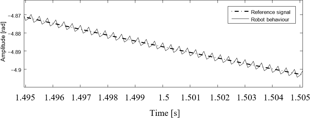
Fig. 11 Zoom into the robot’s third joint tracking the reference with α = 7.2 × 10⁶ and β = 60 × 106.
Figs. 12-14 are dedicated to show the control signal provided by the controller for the first, second and third robot joints respectively, working with the lower limits of the α, β values located in the 3rd range.


The control signal appearing in Fig. 12, has -for the steady state- a frequency of 1000 Hz and an amplitude of 7 × 10⁵ Nm. For the transient stage has a frequency of 280 Hz and evidently it has a variable amplitude coming from 0.85 × 10⁷ to 7 × 10⁵ Nm.
The control signal appearing in Fig. 13, has -for the steady state- a frequency of 2900 Hz and an amplitude of 8 × 10⁵ Nm. For the transient stage has a frequency of 1000 Hz and evidently it has a variable amplitude coming from 0.9 × 10⁷ to 8 × 10⁵ Nm.
The control signal appearing in Fig. 14, has -for the steady state- a frequency of 2500 Hz and an amplitude of 4.85 × 10⁵ Nm. For the transient stage has a frequency of 780 Hz and evidently it has a variable amplitude coming from 0.85 × 10⁷ to 4.85 × 10⁵ Nm.
It is possible to observe a zoom inside a transitional stage from the transient to steady state for both the trajectory tracking in Fig. 15 and for the control signal behaviour in Fig. 16, referred to the second robot link and with high α-β values. These last two figures show that frequency and wave shape are the same for both position and torque, at any time.


Discussion
Results given by experiments performed with α and β located in the upper limit of the 1st range of values in Table 2, supports that, the STA working under the given conditions, causes a loss of system robustness when the chattering is reduced. Figs. 2-4 show that disturbances are not vigorously rejected.
Results given by Figs. 5-7, support that the STA has the capability to totally remove the chattering-effect, being that the control functions are smooth and low in both frequency and amplitude, and this produces a smooth tracking of the reference in steady state with a frequency value near to zero (i.e., the robot does not vibrate in steady state), as it can be observed in Figs. 2-4. Results given by experiments performed with α and β located in the lower limit of the 3rd range of values in Table 2, supports that, the STA working under the given conditions, produces a rise in the level of chattering-effect when the system robustness is increased. Figs. 8-10 show a stronger and faster convergence than that obtained in Figs. 2-4, in addition Fig. 11 does not show disturbances caused by gravity in the nearest of 1.5 s as it is shown in Fig. 4.
As such, the following remarks are obtained:
The chattering can be considered as an amount of energy injected to the control system.
The control system needs energy to maintain robust properties.
A significant reduction of energy, decreases the reaction power to reject disturbances.
According to the first law of thermodynamics, it is impossible maintain robustness when the available energy decreases.
It is important to mention that in this work is not argumented that the STA fails under specific operational conditions, but it just lower the robust properties when it is tuned to produce lower chattering levels.
Simulation results obtained in this research support that for the STA:
Where:
Where:
As a first approach to apply the proposed equation (7), herein is also proposed for practical purposes that the amount of chattering can be measured taken the angular velocity of its behavior, i.e., the amplitude multiplied by the frequency of the tracking error. Further, the inverse of the convergence time is a practical measure of system robustness. Taken this criteria, and the data provided in the last section, the values for k for the values of α and β in the begin of third range of Table 2 can be obtained as:
For the first, second and third robot’s joints respectively. As it can be observed,
equation (7) can be used in many
ways, according to the criteria employed to define the amount of chattering,
robustness, and the values for α and β. Can also
be selected the average of k for a large range of
α and β. A more extensive and deep study to
characterize k is proposed for future works, along with a
thermodynamic approach to measure
Equation (7) is the main result of this work, and it is valid for the given working conditions and for the extended following conditions.
Including an explicit disturbance w in the plant under control, it yields to:
Where:
x is still the vector for the system states, f is a bounded uncertainty, g represents the gain vector for the control for matched/unmatched uncertainties, and y is the system output vector.
The normal form proposed by Isidori, 1989, for (8) includes the transformation:
Where:
Using this reasoning we can infer that results given for the STA can be generalized for control systems including implicit/explicit, bounded/unbounded, and matched/unmatched uncertainties.
Even more, as it can be seen, there is a wide range of values for
In practice, certain ranges of values for α and β parameters of the STA, causes control instability, at least for a robotic plant as that given by (1) and under the specified working conditions. An open problem arising from this work is the mathematical formulation for the STA conditions (α, β values) under which a given control system becomes unstable (see 2nd range in Table 2).
There are implications of results obtained herein in actual practical applications. In most cases in which engineers design robust control systems, SMC is taken into account as a possible solution to deal with perturbed systems, and the aim of designers is to obtain robustness and rejection of chattering at the same time when HOSM are used to control electromechanical plants (with relative degree equals two), as theory claims. This work will help engineers to narrow their expectations in this regard, posing the reality as it is in the practical implementation processes. A typical practical example in which engineers should put special attention, is in serial robotic plants, where each articulation of the robot is disturbed by the chattering-effect produced by neighboring joints, when system robustness is high. Remember that when the robot is operating on industrial environments, it has high robustness requirements.
Conclusions
The STA is a class of HOSM, which is capable to reduce the chattering-effect, however, results obtained in this work show that the drastically reduction of the chattering, reduces significantly the robustness for the control system.
Accordingly with expression (7) the chattering-effect produced by the HOSM can be considered as an amount of energy injected to the control system and a significant reduction of the chattering-effect via the HOSM may give rise to a control signal with low level of energy, and thus decreasing the reaction power in rejecting disturbances. This result is demonstrable at least for the outlined control conditions.

