Creation of the spatial domain

The spatial domain to solve the Richards’ equation was created with the following steps: 1) selection and discretization of domain boundaries, 2) filling of interior regions with uniformly distributed random points, and 3) triangulation with the ^{Delaunay algorithm (1934)}. The two types of existing boundaries are exterior (where the points of interest are in the interior) and interior (where the points of interest are in the exterior).

To model the furrow infiltration, a square boundary was assumed and the upper side was replaced by a periodic function, in this case, a sinusoidal function was chosen, f(x) = 15 sin (πx/45) which gives a 30 cm furrow in height and 90 cm from ridge to ridge (Figure 1). Once the boundary was obtained, the next step was to obtain the discretization of the same.

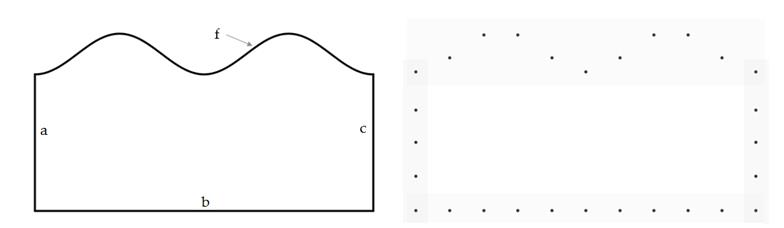
Figure 1 Left: Boundary with the upper part similar to an irrigation furrow. The upper part f is a sinusoidal function translated and scaled to match the upper part of sides a and c. Right: Discretization of the left boundary, boundary points. 

To fill the interior first the smallest square containing all boundary points was obtained. Once this square was obtained C: [a, b] x [c, d] the point P _k was sought by using a uniform distribution within the square C. To find out if P _k was within the boundary, the sum of the angles from P _k of each pair of contiguous boundary points was found (Figure 2 and 3).

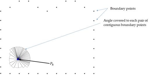
Figure 2 Point P _k within a "furrow"- type boundary. Note that for a point that is in the interior of a boundary, the covered angle is of 360 degrees. 

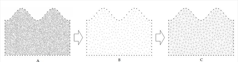
Figure 3 (A) “furrow-type domain” with 10.000 interior points. (B): Domain (1) after removing the points that have a distance less than 5 mm. (C): Domain triangulation (2). 

For a point in the interior of a boundary the sum of the angles mentioned is ± 360 degrees and for a point on the exterior of the boundary the sum is zero degrees. When discarding the exterior points remains a domain (Figure 3(A)). The large number of points in Figure 3 (A) generated in this first step is because the interior regions are required to be as dense as possible. Subsequently, we proceeded to eliminate points that were at a distance considered convenient, for example, all those that were at a distance less than 5 mm from each other (Figure 3 (B)), to finally proceed to the union of the remaining points, resulting in a triangulation of the domain, as shown in Figure 3 (C). The domain with more points will have a greater number of nodes, which implies a greater computational cost to find the solution.

Although the function used to represent a furrow is periodic and a half would be sufficient to model the infiltration, in this study all the exemplification is done using three furrows; this is due to a simulation with different loads in each of the furrows to observe the behavior of the wetting profile.

Finite-Differences Solution for the 2D Richards’ equation

The equation (1) evaluated at some point t in time is written as follow:

In this equation Ψ(k) is a function of three variables Ψ (x, z, t). Equation (1) with discrete time derivative takes the following two forms (in addition to others, depending on the chosen scheme and precision):

Equation (7) corresponds to the explicit model and equation (8) corresponds to the implicit model. Thus, the right side of equation (8) is defined as the operator Op (Ψ _k ), equations (7) and (8) take a simpler form:

when C [Ψ (k)] ≠ 0, the solution obtained is a recursive solution:

However, in the saturated zone C (Ψ _k ) = 0, so that at these points equation (11) cannot be applied. For these cases it is necessary to optimize equation (10) and the algorithm used in this work is that of the conjugate gradient for non-linear problems also called "non-linear conjugate gradient". The method requires that a function to minimize be defined, in this case we require that equation (10) be fulfilled, whereby naturally an error function is as follows:

The non-linear conjugate gradient for 2D Richards

Following the procedure described by ^{Dai and Yuan (1999)}, starting from equation (12) defined as the error function, and with the operator defined from equation (8), the procedure consists of the following steps: 1 ) It was chosen x0=Ψ(k); 2)∆x0=-∇xE(x0); 3)α0=arg⁡minEx0+α∙∆x0; 4) x1=x0+α0∙∆x0 and 5) S0=∆x0 . From step 1 to step 5 is the part where starts x0, the following steps (6 - 10) are iterative and the algorithm ends when Ex0 ” is small: 6)∆xn=-∇xE(xn); 7)β=ΔxnT∙Δxn/Δxn-1T∙Δxn-1; 8)Sn=Δxn+β∙Sn-1; 9) αn=arg⁡minExn+α∙Δxn and 10) xn+1=xn+αn∙Sn. Finally xn+1 is chosen as the solution to the pressures in time t. Although it is possible to apply the algorithm for the whole vector of pressures, for reasons of performance the changes were made only in the saturated zone, because, in the unsaturated zone, it is possible to apply the recurrence rule. The initial condition for x0 is Ψ(k) in the unsaturated zone with the explicit method and Ψ(k-1) in the saturated zone.

Method to solve the operator OpΨk

To simplify the notation the following simplifications were made: Ψi is defined as the pressure in the node i at any time; the spatial coordinate of the node i is defined as Ci=xi,zi, where xi is the coordinate in the length and zi in the depth; Ci,j is the spatial coordinate of the j-th node related to the node i, that is Ci,j = Ci,j=xi,j,zi,j; mj is the number of nodes related to node i and Pi is the ternary xi,zi,Ψi=Ci,Ψi. Using first-order derivation, the derivative in Ci is estimated by deriving the plane a∙x+b∙z+c that best fits the points Pi,P1,i,P2,i,⋯,Pmi,i. One way to approach this plane is to use the pseudoinverse matrix defined by Cj,i and solving for a, b and c ; the points Pi,P1,i,P2,i,⋯,Pmi,i satisfy a∙x+b∙z+c , so a∙xi+b∙zi+c=Ψi, and a∙xi,j+b∙zi,j+c=Ψi,j. The above equations define the following system of equations:

The matrix A of equation (13) is not necessarily invertible, however, on the assumption that any system can be optimized (^{Penrose, 1955}), it is defined as:

where A+ is the pseudoinverse matrix of A.

With values a, b and c obtained, it is possible to derive in any direction, in particular, towards x and z. Similarly to the linear approximation, using a second-order derivation, the derivative in Cj,i was estimated by deriving the surface a∙x2+b∙x∙y+c∙y2+d∙x+e∙y+f that best fit the points Pi,P1,i,P2,i,⋯,Pmi,i. One way to approach this surface is to use the pseudoinverse matrix defined by Cj,i and solving for a, b, c, d, e, and f, thus, we obtained the points Pi,P1,i,P2,i,⋯,Pmi,i satisfying a∙x2+b∙x∙y+c∙y2+d∙x+e∙y+f , so they also satisfy a∙xi2+b∙xi∙yi+c∙yi2+d∙xi+e∙yi+f=Ψi and a∙xi,j2+b∙xi,j∙yi,j+c∙yi,j2+d∙xi,j+e∙yi,j+f=Ψi,j. These equations are defined as follows:

where applying the same consideration as in the solution of equation (14), the matrix A is defined as:

where A+ is the pseudoinverse matrix of A.

At the end of this procedure, with the values a, b, c, d, e, and f obtained, the derivative was calculated.

Calculation of the infiltrated water depth

The volume infiltrated per length unit of channel in the unit time (A˙I) was calculated with the following expression (^{Fuentes, De León-Mojarro, & Hernández-Saucedo, 2012}):

where qIx,y,z,t is the infiltration flow per unit of channel surface or unit flow and Pm is the wetted perimeter in each furrow.

Comparison between the implicit schema and the mixed scheme

The two schemes (implicit and mixed) were compared. The values used were from the Montecillo soil (^{Fuentes, 1992}; ^{Saucedo, Zavala, & Fuentes, 2011}; ^{Saucedo et al., 2013}), that were: θr=0.0000cm3cm-3 , θs=0.4865cm3cm-3 , Ks=1.8400cmh-1, Ψd=-45.9000cm, m=0.1258 and a depth L=90cm. In this simulation, we used an average distance between nodes in both schemes of Δz=1 cm, and a time discretization of Δt=0.01 h for the mixed method, whereas for the implicit an Δt=0.00128 h was used. The results for 240 min (Figure 4) indicate no difference between the two schemes but the mixed scheme requires a much finer time discretization than the implicit scheme. However, the implicit scheme requires more calculations for each time, which makes the simulation of an infiltration event a little slower.

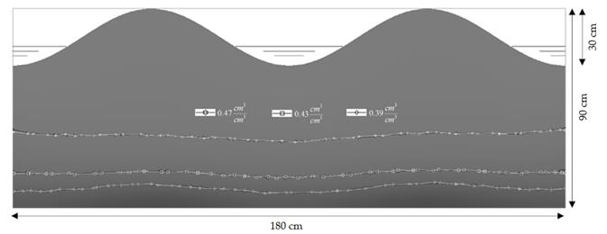
Figure 4 Comparison between the implicit scheme (white lines) and the mixed scheme (black lines) at 240 minutes. 

The computation time required to simulate the 240 min, using a computer of 6 GB in RAM, for the mixed method was of 18 min, whereas for the implicit method it was of approximately 24 min, that is, the implicit method required 30% more time than the mixed method, however, with today's computing resources the simulation time can be reduced a bit more.

It is important to mention that this computation time corresponds to the discretization of the three furrows, if this simulation is conducted only in half of a furrow, times to get the solution would be reduced, with the same spatial and time discretization, at 4, 5 and 6 minutes, respectively. The result of the infiltration curves of the solutions are practically the same.

Simulation of furrow infiltration in 2D: constant depths in furrows

Based on the hydrodynamic characteristics of the Montecillo soil, a simulation of the infiltration process was performed in three furrows in which a 10 cm water depth was applied in the first and third hours of infiltration, and in the second and fourth hour, 5 cm of depth. Curves were drawn with the following volumetric water contents: 0.47 cm ³ cm ^-3, 0.43 cm ³ cm ^-3, 0.39 cm ³ cm ^-3, 0.35 cm ³ cm ^-3, 0.31 cm ³ cm ^-3. Figure 5 shows two moisture profiles corresponding to the first hour of infiltration, at minute 60 water depth changes from 10 cm to 5 cm. As can be seen, the wetting front moves faster in the first hour (Figure 5) than in the second one (Figure 6) because in the second hour there is a 5 cm water depth from the base of the furrow, so, in that hour, the effects of capillarity contribute more than the pressure effects. The inverse effect can be seen in the upper image of Figure 7, in which the downward pressure is greater than in the previous minutes, because water depth changed to 10 cm in the minute 120.

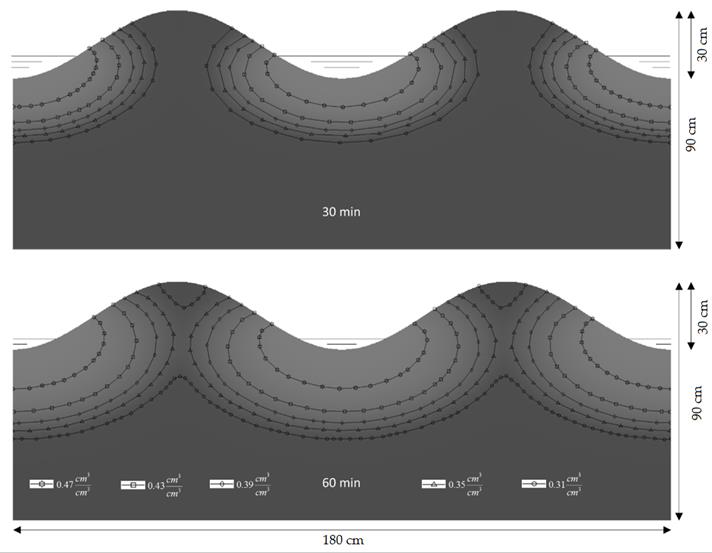
Figure 5 First hour of infiltration with a 10 cm depth from the base of the furrow. At minute 60 the depth changes to 5 cm. 

Figure 6 Moisture distribution during the second and first hour. The 5 cm depth is constant. 

Figure 7 Moisture distribution in the third and fourth hour. 

Figure 6 shows two moisture profiles corresponding to the second hour of infiltration and Figure 7 shows two moisture profiles corresponding to the third and fourth hour. As can be seen in the series of images, when the change of water depth from 10 to 5 cm in the furrow is made, it favors the wetting in the ridges of the furrow, whereas with a higher depth, the redistribution of the moisture profile is higher at the base of the furrow than in the ridge. With a simulation time of 60 minutes, it is already possible to carry the moisture content to 0.31 cm³ cm^-3 in a depth of 35 cm and the ridges of the furrow.

The moisture content in the furrow at 180 minutes of simulation can be seen that it is practically saturated: that is, it has an amount of water slightly higher than 0.47 cm³ cm^-3 and the maximum amount of water it can have is 0.4865 cm³ cm^-3. After 135 min the top of the furrows are saturated and, from that moment, for any moisture content in the soil profile tends to be horizontal, which resembles a constant infiltration (Figure 7).

Simulation of furrow infiltration in 2D: different depths in furrows

Using the same hydrodynamic characteristics of the Montecillo soil of the previous section, a simulation was performed in three furrows where in each of them the loads were now different: 3, 9 and 6 cm, from left to right. The simulation results showed that the redistribution of moisture in the ridges of the furrow and on the soil profile during the infiltration process is better in the area between the furrows with water depth of 9 and 6 cm (Area 1) than that between furrows with 3 and 9 cm of water depth (Area 2) (Figure 8 and Figure 9).

Figure 8 Moisture distribution in the first and second hour. 

Figure 9 Moisture distribution in the third and fourth hour. 

The moisture distribution in the ridges of the furrows, the union of the wetting bulbs and wetting area is better in the first area than in the second. In area 1, the furrow that has 9 cm of water depth must contribute more water to the furrow on the left (3 cm water depth), so that the distribution of moisture to lower layers is less than between furrows of 9 and 6 cm.

Also, the moisture content in the ridge of the furrow with water of 9 cm is higher than in the ridge of the furrow with 3 cm, in the latter the main problem is that the wetting towards the lower layers (Figure 9) is delayed. This problem is very common in the events of gravity irrigation, where the flow rate applied in each furrow is not homogeneous due to the fact that the siphons are not calibrated, that there are faults in the opening of gates or, as in most cases, the expense provided in each furrow is at the discretion of the irrigator. This brings several complications, among the most important is that the water depth applied in each furrow is not homogeneous, which leads us to apply more water than that needed in some parts of the plot, or in the worst case, to apply a smaller amount.

As a problem in two dimensions, the infiltrated water table is now represented as the infiltrated area, which, if multiplied by a length, the infiltrated volume is obtained. Thus, the infiltrated area (cm ²) was calculated in each furrow with equation (17) and by making comparisons (Figure 10), one can see that for the time of 240 min in the furrows of 9, 6 and 3 cm of each water depth, infiltrate on average 512, 467 and 401 cm ² respectively. That is, 110 cm ² less would be infiltrating in the furrow with load of 3 cm, moreover, the furrows with a higher depth will tend, by difference in the depths, to contribute to the wetting of the furrows with less depth, which also brings with it a reduction in the wetting pattern in each one of the furrows that corresponds them to wet.

Figure 10 Evolution of the infiltrated water table in furrows with variable load