


Serviços Personalizados
Journal
Artigo
 texto em
  Inglês (pdf)
 Artigo em XML
 Referências do artigo
 Enviar este artigo por email
Indicadores
-
 Citado por SciELO
 -
 Acessos
Links relacionados
-
 Similares em
SciELO
Similares em
SciELO
Compartilhar

 Permalink
Tecnología y ciencias del agua
versão On-line ISSN 2007-2422
Tecnol. cienc. agua vol.9 no.5 Jiutepec Set./Out. 2018 Epub 24-Nov-2020
https://doi.org/10.24850/j-tyca-2018-05-05
Articles
Geostatistical estimation of the spatial distribution of mean monthly and mean annual rainfall in Nuevo León, Mexico (1930-2014)
1Instituto Nacional de Estadística y Geografía (INEGI), silvio.villarreal@inegi.org.mx
2Instituto Mexicano del Petróleo (IMP), mdiazv@imp.mx
Considering the strong spatial variability of precipitation in the state of Nuevo León, Mexico, geostatistical techniques such as ordinary kriging and stochastic simulations were applied to estimate the spatial distribution of annual and seasonal mean precipitation from 1930 to 2014. The data set corresponds to 95 weather stations with at least 25 years of records and includes neighboring stations of the NOAA and states bordering Nuevo León. Application of a systemic approach enabled establishing isotropic and anisotropic models (variograms) to represent the spatial dependence of rainfall data. Estimations and simulations were obtained by applying modeled variograms. In order to assess the estimation quality, a cross-validation technique was applied. Considering the spatial variability and data quality, the estimation results are consistent with the observed seasonal rainfall patterns corresponding to north and northeastern Mexican climatic regions.
Keywords Geostatistics; spatial estimation; rainfall; kriging; simulations; anisotropy; Nuevo León
Considerando la fuerte variabilidad espacial del fenómeno de la precipitación en el estado de Nuevo León, México, se utilizaron las técnicas geoestadísticas de kriging ordinario y simulaciones estocásticas, con el objetivo de estimar la distribución espacial de la precipitación media anual y para las estaciones de mayor precipitación (primavera y verano). Los datos para el estudio corresponden a 95 estaciones climatológicas, con al menos 25 años de registro en el periodo comprendido de 1930 a 2014, se incluyen datos de estaciones vecinas de la NOAA y estados colindantes a Nuevo León. El uso sistemático de estas técnicas permitió establecer la dependencia espacial de los datos de precipitación, por medio de modelos variográficos isotrópicos y anisotrópicos, los cuales se aplicaron en las estimaciones y simulaciones. Para evaluar la calidad de las estimaciones obtenidas se aplicó la técnica de validación cruzada. Los resultados obtenidos son consistentes con el comportamiento estacional de la precipitación en las regiones climáticas del norte y noreste de México, considerando su variabilidad espacial, y la disposición y calidad de la información de las estaciones climatológicas en el área de estudio.
Palabras clave geoestadística; estimación espacial; precipitación; kriging; simulaciones; anisotropía; Nuevo León
Introduction
Knowledge of spatial distribution is important to hydrology, agriculture and climatology. In hydrology, it serves as input to hydrological modeling for the prediction of extreme events such as surface water flow and floods. Seasonal rainfall is very important to evaluate the effect on the agricultural sector (Englehart & Douglas, 2000), especially in seasonal agriculture since that is highly vulnerable to interannual and seasonal rainfall variability. No doubt climate change has direct impacts on the precipitation regime, and therefore, it also impacts the management of water resources. Hence the importance of studying the spatial and temporal pattern of precipitation changes.
The data used for this study was taken from the network of weather stations belonging to the National Water Commission (CONAGUA, Spanish acronym), and NOAA (National Oceanic and Atmospheric Administration), in the state of Nuevo León. These stations are unevenly distributed, and in some cases the available information is insufficient to characterize the high variability of rainfall and its spatial distribution. Therefore, it is necessary to estimate rainfall in areas where no information is available, using data from neighboring stations. Several authors, such as Goovaerts (1999), Miras-Avalos, Paz-gonzalez, Vidal-vazquez and Sande-Fouz (2007) and Coulibaly and Becker (2007), have shown that geostatistical methods provide better estimates of precipitation than other techniques.
The main objectives of this study are:
Analyzing and modeling the spatial variability of mean monthly and annual precipitation.
Obtaining surfaces of estimate and their errors, using ordinary kriging and Gaussian sequential simulation techniques, for the annual average and higher rainfall months, grouped in two seasonal periods in Nuevo Leon, Spring (February 16.8 mm - May 55.6 mm) and Summer (June 64.8 mm - September 117.7 mm).
Evaluating the results of the approaches used.
Study area and data
The distribution of precipitation in Mexico varies in space and time. It differs throughout the year, geographically increasing north-south due to the effect of latitude. It is also largely determined by the proximity to the Pacific Ocean and Gulf of Mexico (Campos-Aranda, 1998), the orography and atmospheric circulation characteristics (García, 2003).
Nuevo León is located in northeast Mexico, between the Meridian 98° 26' and 101° 14' West longitude, and the parallel 23° 11' and 27° 49' latitude North (Figure 1). Its surface is around 64 000 km2 and the climate is dry. There are three physiographic provinces crossing it partially, the Sierra Madre Oriental, the Great Plains of North America and the Gulf coastal plain. The altitude ranges between 70 and 3 500 meters.
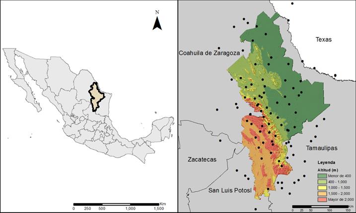
Figure 1 Location of the study area and distribution of weather stations used to estimate rainfall in Nuevo León, Mexico.
The dry and semi-dry climates are located mainly in the northeastern region, along the Great Plains of North America, and southwest of the Sierra Madre Oriental. Semi-warm, temperate and semi-tropical climates have been registered in the center and southern portions of the state of Nuevo León and in a large part of the San Juan River basin(INEGI, 1986), as shown in Figure 2.

The rainfall in the study area is strongly dominated by seasonal variability, since the region is affected by strong rains from tropical storms and hurricanes, due to its proximity to the Gulf of Mexico, and the effect of cold fronts. In general, precipitation is scarce, although there are some places with 1 100 mm. The annual average for Nuevo León was 541 mm over the period of study.
To integrate accumulated monthly and annual rainfall data, the period from 1930 to 2014 was chosen. For each of the weather stations used, at least 25 years of records were considered. In order to have greater spatial coverage, 95 stations were selected taking into account an average distance of 50 km from the Nuevo León border, 56 stations were located in Nuevo León, 11 in Coahuila, 17 in Tamaulipas, 4 in San Luis Potosí, 1 in Zacatecas, and 6 were in Texas (United States of America) (Figure 1). The data sets for PMA , Spring and Summer variables were derived from these stations.
Methodology
The application of the geostatistical methodology to a data set involves three steps: exploratory data analysis, structural analysis and estimation and/or simulation. In the exploratory analysis, quality control processes and criteria for the integration of climate data series were applied based on “Calculation of monthly and annual 30-year standard normals” (WMO, 1989) and “Guide to Climatological Practices” (WMO, 2011), published by the WMO (World Meteorological Organization). The basic statistics for the integrated monthly and annual data were analyzed. The structural analysis focused on knowledge of the spatial variability of the data, the presence of anisotropy was evaluated and the variographic models were obtained for each variable. These models were validated using the cross-validation technique. The third stage involved estimation and simulation, in which the interpolated surfaces were obtained. In this project, in addition to ordinary kriging, the Gaussian sequential simulation technique was applied, which consists of obtaining a new simulated value from a probability distribution function, using sampled values and previously simulated values in a given neighborhood, applying a kriging technique (Chilès & Delfiner, 1999).
Results
Exploratory Analysis
The quality control applied to the data consisted of evaluating the following points:
Spatial Consistency - The coordinates of eight stations were updated due to inconsistency in their location: five in Coahuila (5016, 5032, 5035, 5048 and 5049) and three in Nuevo León (19012, 19054 and 19069).
Format - Improbable dates and repeated records were excluded, as an example in NOAA records, every month of every year has a 31-day format.
Completeness - For the annual data integration, 95 stations were selected that contained at least 25 years of records, considering the criterion of excluding the months with more than five missing daily records or more than three continuous daily records.
The basic statistics for the variables PMA Spring and Summer are described in Table 1. The three precipitation variables have a positive asymmetric distribution, so it is necessary to evaluate whether the "proportional effect" is presented in these cases, which is a particular form of heteroscedasticity (the variability of the data changes throughout the study area), particularly for positive asymmetric distributions, the local variance increases as its local mean increases (Goovaerts, 1997). This proportional effect makes it impossible to interpret experimental variograms (Grimes & Pardo-Igúzquiza, 2010).
Table 1 Basic statistics for variables analyzed. SD (standard deviation), CV (variation coefficient).
To identify how changes in local variance are related to changes in the local
average, it is common to use scatter plots, calculated from mobile windows
(Goovaerts, 1997). Statistics for
mobile windows were calculated with an area of 100 km2, with an
overlap of 25 km2, and 18 were selected, including at least 10
data. The overlap of the windows implies that some data were used repeatedly
for the calculation of local means and variances, which is not relevant at
the moment in which we only want to establish whether or not the
proportional effect exists (Isaaks &
Srivastava, 1989). The result obtained for
PMA
and
Summer
shows that variances and local averages have low correlation (

As is known, the weather stations are located in places where certain characteristics are available in terms of operation and registration, so there are areas with higher concentrations (clustering), particularly when combining the proportional effect and the grouping of the sample data. This led to conflicts with the interpretation of the experimental variograms. One way to know the grouping and the proportional effect is by graphing the local means and variances as a function of distance (Goovaerts, 1997).
For the case of the three variables, fluctuation around a unit value is observed, concluding that the variances and the means are not significantly affected by distance, so there is no need to perform any process to consider the effect of grouping, for example, using only regularly spaced data (Goovaerts, 1997). Figure 4 presents the results obtained for PMA.

Structural analysis
Considering that asymmetry and atypical data directly affect the modeling of variograms, a logarithmic transformation was applied to reduce the degree of asymmetry and analyze the behavior of atypical data. The logarithmic transformation used for Spring did not improve the distribution, so its application was not considered. Figure 5 shows the experimental variograms for the variables with moderate asymmetry ( PMA and Summer ). Their logarithmic transformation were included in the same graph after re-scaling the variance. The logarithmic variograms seem less erratic, with less nugget for PMA ; therefore, this variable is modeled without transformation, while Summer justifies the transformation due to the notable difference between the variograms.
The anisotropy analysis was performed by inspecting the experimental variograms in different directions: 0° (NS), 45° (NE-SW), 90° (EW) and 135° (NW-SE) with an angular tolerance of ± 22.5° (Wackernagel, 2003). Since a portion of the Sierra Madre Oriental is located in the study area, and it influences precipitation patterns, variograms were constructed in the NW20° direction, in association with the regional structure of that mountain range, as well as the perpendicular direction to it (NE70°). Additionally the omnidirectional variogram was constructed (0° direction and angular tolerance of 90°). Gstat software (Pebesma & Wesseling, 1998) and the RGEOESTAD (Díaz, Hernández, & Mendez, 2012) were used to perform this analysis.
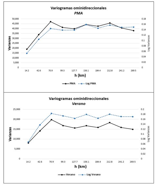
Figure 5 Omnidirectional experimental variograms for PMA and Summer. The logarithms variogram was re-scaled to the variance from the original data.
According to Figure 6, given the inflection points shown in the experimental variograms, two spatial variation scales in the NE70° direction (perpendicular to the structure of the Sierra Madre Oriental) are seen: one with a range of 75 km and another of 125 km approximately. At a distance greater than 125 km, the structure of the variograms becomes erratic in that direction due to the decrease in the number of pairs that contribute to the values of the variances. For the NW20° direction, the variograms show greater spatial continuity (less variance) and follow a pattern similar to the omnidirectional variogram.
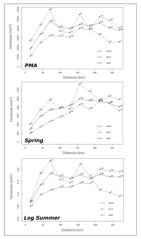
Figure 6 PMA, Spring and Log Summer variograms in NE70°, NW20° directions with angular tolerance of 22.5 (dashed lines), and the omnidirectional variogram (0°) with angular tolerance of 90° (continuous line). The numeric labels show the number of pairs.
Another way to evaluate anisotropy is through the elaboration of a variographic map (Isaaks & Srivastava, 1989), in which the values of the experimental variogram are plotted and the center of the map corresponds to the origin of the variogram. Figure 7 shows a preferential direction towards the NW-SE for Log Summer and PMA, roughly aligned with that presented by the Sierra Madre Oriental. For the case of Spring, this preferential direction appears to be less.

Taking into account the results of the variographic maps, the anisotropic models were used for the variables PMA and Log Summer .
Once the directions of the variograms were defined, spherical theoretical models were adjusted using least squares technique. This procedure was carried out with the RGEOESTAD (Díaz et al., 2012) and gstat (Pebesma & Wesseling, 1998) software, from which variographic parameters were obtained (nugget, sill and range). Table 2 shows the summary and Figure 8 illustrates the adjusted spherical models, including the omnidirectional. The models adjusted for the NE70° direction are not shown in this paper.
Table 2 Variographic parameters NW20°, NE70° and omnidirectional, modeled for Spring, PMA and Log Summer variables.
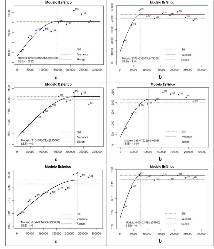
Figure 8 Directional variograms adjusted for PMA , Spring and Log Summer : a) NW20° direction, b) omnidirectional.
All variograms for the NW20° direction exhibit a linear behavior at the origin, as well as small nugget effects, with nugget/sill proportions from 16% to 23%, and represent an origin discontinuity that is attributable to measurement errors and variation at lower distances in the sampling interval (28.4 km).
The variograms in the NE70° direction were modeled to obtain the anisotropy
factor
Cross-validation
The cross-validation technique consists of taking an observation and estimating its value with the remaining observations. This is done repeatedly until all observations are concluded.
The errors are defined as the difference between the observed and estimated values, and are calculated using the following expression:
Where
There are different indicators to measure the quality of the estimate globally. In this work, the following were applied:
Table 3 shows the validation results.
According to RMSE from cross-validation, the anisotropic model improved the PMA and Spring estimations. For the Summer estimation, the isotropic model was better, according to the results.
Estimation and Simulation Methods
The estimated rainfall and error maps are shown in Figures 9, 10 and 11. These maps were generated using the ArcMap software with geostatistical analyst extension (ESRI, 2016), using previously adjusted variographic models and applying the ordinary kriging and Gaussian sequential simulations techniques. These techniques are discussed and widely analyzed in the works of some authors such as: Chilès and Delfiner (1999), Goovaerts (1997), Wackernagel (2003) and Isaaks and Srivastava (1989).
Isotropic variographic models were used for the Gaussian sequential simulation technique, applying an anamorphosis transformation to the data. The open source program gstat (Pebesma & Wesseling, 1998) was used to perform 100 simulations for each of the variables and to generate the maps. An average of these simulations was considered, using the ArcMap geostatistical analyst extension (ESRI, 2016).
The anisotropic model better reproduced the spatial distribution of PMA rainfall data, emphasizing the preferential direction to the Sierra Madre Oriental. In the northern part of Nuevo León, there are very similar patterns among the three models (isotropic, anisotropic and simulations), and as is to be expected, the simulations reproduced the exact same extreme data values.
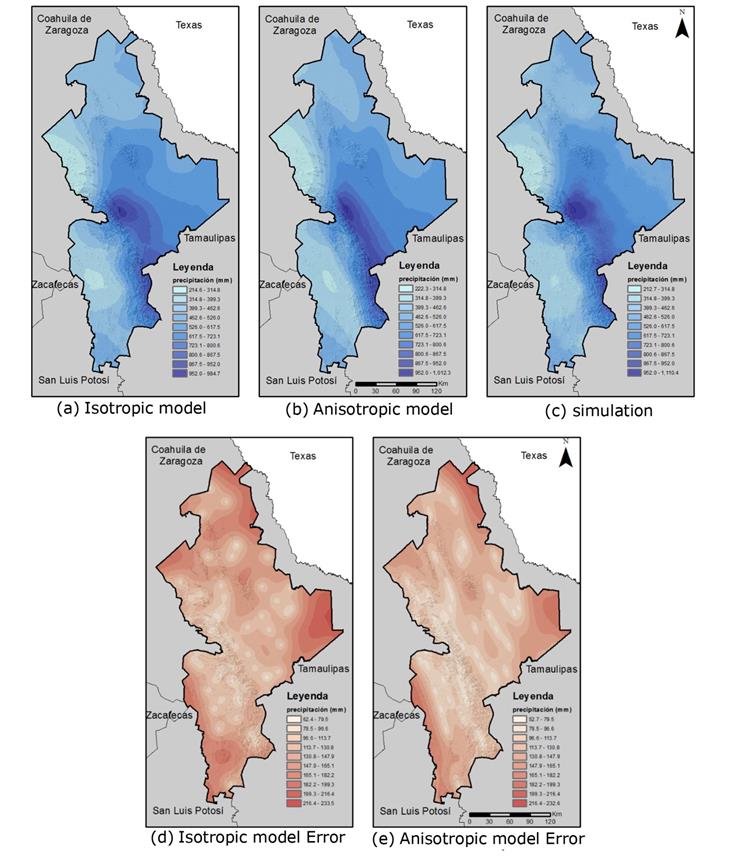
Figure 9 Nuevo León maps: estimation, simulation and estimate error for PMA , in the period 1930-2014.
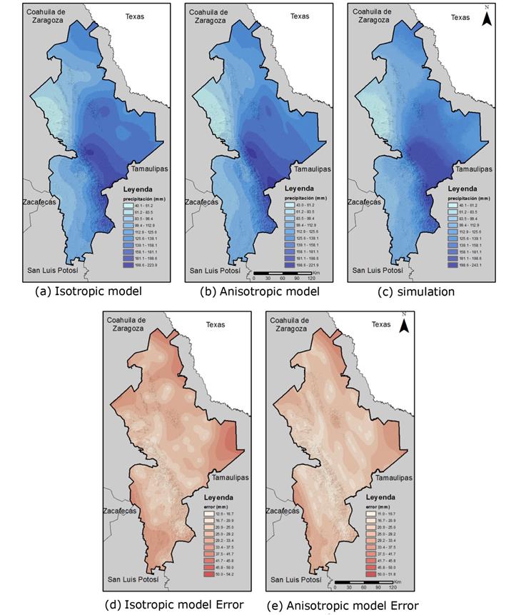
Figure 10 Nuevo León maps: estimation, simulation and estimate error for Spring , in the period 1930-2014.

Conclusions
The use of geostatistical techniques enabled developing isotropic and anisotropic variographic models of spatial dependence for precipitation data. These models were fundamental to the application of ordinary kriging and gaussian sequential simulations.
The seasonal precipitation patterns for the state of Nuevo León were much better using gaussian sequential simulations, given the presence of cyclonic events in the Caribbean Sea and the Gulf of Mexico, with a dominant NW-SE direction and with values higher than 40 mm. These values contrast with the results of average monthly precipitation interpolated with regression techniques for Bravo-Conchos Rio Hydrological Region 24, which covers a portion of the state of Nuevo León (Nuñez-López, D., Treviño-Garza, E., Reyes -Gómez, V., Muñoz-Robles, C. Aguirre-Calderón, O. & Jiménez-Pérez, J., 2013), finding high values during the rainy months, predominantly in the highlands of the eastern Sierra Madre. However, it is not possible to clearly identify the high precipitation values in the vicinity of the Monterrey metropolitan area, in the territorial portion of the North Gulf Coastal Plains physiographic province, perhaps due to the quantity and/or distribution of the weather stations used.
On the other hand, in relation to the maximum annual average precipitation values obtained, the citrus region is notable, comprised by the Allende, Montemorelos, Hualahuises, General Terán and Linares municipalities. This territorial area corresponds to the North Gulf Coastal Plains physiographic province, in addition of the municipality of Santiago, and belonging to the province of the Sierra Madre Oriental, whose precipitation values range between 800 and 1 110 mm, according to the range (800 to 1 200 mm) reported by Vidal (2005).
Given the RMSE values obtained by the cross-validation, the use of the anisotropic models improved the estimates for PMA and Spring, while for Summer the isotropic model was better. In all cases, the improvement is insignificant, so the isotropic model was chosen for the simulations.
Although the processing time was longer in the Gaussian sequential simulations, its use is recommended because the precipitation patterns were better defined than ordinary kriging.
The incorporation of weather stations from states adjacent to Nuevo León, including those of the NOAA in Texas, contributed to greater and better spatial coverage, which enabled obtaining sufficient information to make the estimations throughout the Nuevo León territory.
Acknowledgment
We thank the National Institute of Statistics and Geography (INEGI) for the support given to the preparation of this project. We also thank Juan Antonio, Diana and Carlos for their valuable suggestions and invaluable support.
REFERENCES
Campos-Aranda, D. F. (1998). Procesos del Ciclo Hidrológico. San Luis Potosí, México: Universidad Autónoma de San Luis Potosí. [ Links ]
Chilès, J. P., & Delfiner, P. (1999). Geostatistics: Modeling Spatial Uncertainty (2nd ed.). New York, USA: John Wiley & Sons Inc. [ Links ]
Coulibaly, M., & Becker, S. (2007). Spatial interpolation of annual precipitation in South Africa. Comparison and evaluation of methods. Water International, 32(3), 494-502. [ Links ]
Díaz, M., Hernández, V., & Méndez, J. (2012). RGEOESTAD. México, DF, México: Instituto de Geofísica, Universidad Nacional Autónoma de México. Recuperado de http://mmc2.geofisica.unam.mx/gmee/paquetes.html y http://mmc2.geofisica.unam.mx/gmee/grupo_md.html [ Links ]
Englehart, P. J., & Douglas, A. V. (2000). Dissecting the macro-scale variations in Mexican maize yields (1961-1997). Geographical and Environmental Modeling, 4(1), 65-81. DOI: 10.1080/136159300111379 [ Links ]
ESRI, Environmental Systems Research Institute. (2016). ArcMap- Geostatistical Analyst Extension version 10.5. Inc. Red Lands, California. [ Links ]
García, E. (2003). Distribución de la precipitación en la República Mexicana. Investigaciones Geográficas, 50, 67-76. [ Links ]
Goovaerts, P. (1997). Geostatistics for Natural Resources Evaluation. New York, USA: Oxford University Press. [ Links ]
Goovaerts, P. (1999). Geostatistics in soil science: State-of-the-art and perspectives. Geoderma, 89(1-2), 1-45. [ Links ]
Grimes, D., & Pardo-Igúzquiza, E. (2010). Geostatistical analysis of rainfall. Geographical Analysis, 42, 136-160. [ Links ]
INEGI, Instituto Nacional de Estadística y Geografía. (1986). Síntesis Geográfica del Estado de Nuevo León. México, DF, México: Secretaría de Programación y Presupuesto. [ Links ]
Isaaks, E. H., & Srivastava, R. M. (1989). An Introduction to Applied Geostatistics. New York, USA: Oxford University Press . [ Links ]
Mirás-Avalos, J. M., Paz-González, A., Vidal-Vázquez, E., & Sande-Fouz, P. (2007). Mapping monthly rainfall data in Galicia (NW Spain) using inverse distances and geostatistical methods. Advances in Geosciences, 10, 51-57. [ Links ]
Núñez-López, D., Treviño-Garza, E., Reyes-Gómez, V., Muñoz-Robles, C., Aguirre-Calderón, O., & Jiménez-Pérez, J. (2013). Interpolación espacial de la precipitación media mensual en la cuenca del río Bravo/Grande. Tecnología y Ciencias del Agua, 4(2), 185-193. [ Links ]
Pebesma, E. J., & Wesseling, C. G. (1998). Gstat, a Program for Geostatistical Modelling, Prediction and Simulation. Computers & Geosciences, 24, 17-31. [ Links ]
Vidal, Z. R. (2005). Las Regiones Climáticas de México. México, DF, México: Instituto de Geografía, Universidad Nacional Autónoma de México. [ Links ]
Wackernagel, H. (2003). Multivariate Geostatistics: An introduction with Applications. Springer-Verlag Berlin Heidelberg New York. [ Links ]
WMO, World Meteorological Organization. (1989). Calculation of Monthly and Annual 30-Year Standard Normal. WDCP-No. 10, WMO-TD/No. 341, Geneva: World Meteorological Organization, 11p. [ Links ]
WMO, World Meteorological Organization. (2011). Guide to Climatological Practices. WMO-No.100, Geneva: World Meteorological Organization, capítulo 3. [ Links ]
Received: June 09, 2017; Accepted: April 03, 2018
 Este es un artículo publicado en acceso abierto bajo una licencia
Creative Commons
Este es un artículo publicado en acceso abierto bajo una licencia
Creative Commons
