


 nova página do texto(beta)
 Inglês (pdf)
 Artigo em XML
 Referências do artigo
 Enviar este artigo por email
 Citado por SciELO
  Similares em
SciELO
Similares em
SciELO 
 Permalink
Introduction
Climate analysis is essential to identify climate change processes in different areas. These analyzes intend to identify variations in the climatic variables (temperature and precipitation) concerning the normal values recorded (historical averages) (Amador&Alfaro, 2009). According to the Intergovernmental Group of Experts on Climate Change (IPCC) (IPCC, 2007), climate variability is associated with natural processes on the planet that act at different scales (diurnal, seasonal, interannual and interdecadal). Only those variations in climate that persist systemically and sustainably for extended periods (decades or longer periods) are considered signs of climate change. Similarly, these changes may be due to natural cyclical processes, physical processes such as changes in the radiative balance, or external forcings of anthropogenic origin (IPCC, 2007; Amador&Alfaro, 2009).
At the international level, the climate change discourse states that in the last 100 years, global temperatures have gradually increased due to the emission of greenhouse gases (IPCC, 2007). These increases have accelerated over the past 30 years, setting off increases in the frequency and intensity of temperature extremes (Houghtonet al., 2001; Alexanderet al., 2006; Alexander, 2016). The increase in temperature anomalies also implies alterations in precipitation (due to ocean warming and variations in wind behavior). Consequently, a greater frequency of hydro-meteorological phenomena could affect biological and human communities (IPCC, 2014; Alexanderet al., 2019). Antecedents in Mexico mention that since 1970 there has been a significant increase in maximum temperature between 1 and 3 ºC in the northwestern region (Gutiérrez-Ruacho, O. et al., 2010; Lobato-Sánchez&Altamirano-del-Carmen, 2017). According to climate change scenarios, this trend is expected to continue in the country (Condeet al., 2011; Magañaet al., 2012), causing that the warm zones become the most vulnerable due to the increase in mean temperature.
Therefore, climate variability and its causes are the main elements to consider in climate change vulnerability studies (Tonmoy et al., 2014). As a complex topic, the analysis of climate variation is usually presented descriptively, which is difficult to integrate with other vulnerability components, which are generally expressed in assessment indicators (Tonmoy et al., 2014; Nájera & Carrillo, 2022). For this reason, one way to synthesize climate variability analyses is by indices (Vázquez, 2010). There are different validated indices (Alexander, 2016), most of them derived from the one proposed by the World Meteorological Organization (WMO) through the Expert Team on Climate Change Detection and Indices (ETCCDI) (Zhang, 2011), built with indicators working with daily data. However, in most Mexican territory, the largest and oldest network of weather stations only makes available to the public information from daily data collection compiled into monthly data (due to the loss of information that arises during daily collection) (Luna et al., 2018). While this is not a persistent condition throughout the country, most weather stations that maintain the daily data quality restrict their information to public access. Also, the information in global estimation databases such as WorldClim 2.1 is presented in monthly compilations.
In this sense, the objective of this research was to construct and validate a climate variability index composed of functional indicators based on monthly data, applied to warm climates, using a fragment of the Pacific Coastal Plain region as a case study.
Material and Methods
To construct the indicators, we used the method described by Nardo et al. (2005). This method comprises two processes; conceptual analysis (choice of dimensions based on reference research) and operational analysis (definition of indicators and their application in a case study for statistical validation).
Conceptual analysis
For choice the dimensions, we follow the recommendations of the reviews of research applied to Mexico made by Jiménez (2011) and Amador & Alfaro (2009). Jiménez (2011) states that a practical way to section climate indicators is according data measurement units. For example, indicators based on air temperature, indicators based on precipitation, and correlation climate indicators that measure the relationship of temperature and precipitation with global signals of natural climate variation originating from the ocean-atmosphere interaction, mainly for Mexico the Pacific Decadal Oscillation (PDO) and El Niño-Southern Oscillation (ENSO). In this way, conflicts for data measurement units are minimized, and the analysis is based on the general variations in temperature and precipitation and the possible influence of global signals on these variations.
Amador & Alfaro (2009), in a more complex way, propose that according to the scale of the data, the indicators can be grouped into six dimensions: 1) weather (indicators of climatic variables during the day); 2) climate (indicators that measure temperature and precipitation extremes and averages over a series of years); 3) variability (indicators that measure temperature and precipitation anomalies over a series of years); 4) planetary variability (indicators of the teleconnection of temperature and precipitation with global signals of natural climate variation derived from ocean-atmosphere interaction such as PDO and ENSO); 5) climate change (indicators that measure the relationship with extreme events); and 6) climate change scenarios (indicators that measure the difference between the scenario and the current climate). Although this classification may cause conflicts for data measurement units, it is a complete way of analyzing climate variability from the different scales of climate activity.
We chose the data scale proposed by Amador & Alfaro (2009) as the central axis for defining dimensions. Therefore, excluding the weather dimension (due to the lack of daily climate data), five dimensions were established: 1) climate; 2) climate anomalies; 3) natural climate variability teleconnection; 4) extreme events; 5) long-term climate change. Incorporating Jiménez's (2011) conclusions, we determined that the indicators obtained from the operational analysis were grouped into variables according to the data measurement units.
Operational analysis
To define the indicators, we analyzed the indicators implemented to assess climate variability in vulnerability studies on climate change in Mexico from the literature review by Nájera&Carrillo (2022) (Monterrosoet al., 2012; Bacaet al., 2014; Rivas&Montero, 2014; Ahumada-Cervanteset al., 2015; Monterrosoet al., 2018) and their references (Martínez&Patiño, 2010; Zhang, 2011; Fernándezet al.,2012; Fernándezet al.,2014; Arreguínet al., 2015; De la Moraet al., 2016; Figueroa-Gallegos, 2017). We choose the most recurrent indicators that could be integrated into the dimensions previously established in the conceptual analysis. Other indicators suggested in Jiménez (2011) and Amador&Alfaro (2009) were included. In total, 48 indicators were defined, grouped into 12 variables and five dimensions. We maintained a balance of two to three variables per dimension and three to four indicators per variable (Table 1).
Table 1 Proposed indicators for the climate variability index from monthly data (description, units, and authors are specified in the extensive table in Annex 1)(Annex 1) .
| Dimension | Variable | Indicator |
|---|---|---|
| 1. Climate | Climate variables | Annual mean temperature (Tp) of the period |
| Maximum temperature (Tmax) of the period | ||
| Minimum temperature (Tmin) of the period | ||
| Average annual precipitation (PP) of the period | ||
| Extremes of climate temperatura | Maximum temperature of the monthly highs | |
| Minimum temperature of monthly minimums | ||
| Number of summer months | ||
| Number of tropical months | ||
| Extremes of climate precipitation | Maximum annual accumulated monthly precipitation | |
| Simple monthly intensity precipitation index | ||
| Dry months index | ||
| Annual average of months with precipitation | ||
| 2. Climate anomalies | Anomaly index | Average temperature anomaly index in the period |
| Maximum temperature anomaly index in the period | ||
| Minimum temperature anomaly index in the period | ||
| Accumulated annual mean precipitation anomaly index for the period. | ||
| Incremental anomalies | Annual average temperature anomaly index >5 % | |
| Annual maximum temperature anomaly index >5 % | ||
| Annual minimum temperature anomaly index >5 % | ||
| Accumulated annual mean precipitation anomaly index >5 % | ||
| Decrement anomalies | Annual average temperature anomaly index <5 % | |
| Annual maximum temperature anomaly index % <5 % | ||
| Annual minimum temperature anomaly index <5 % | ||
| Accumulated annual mean precipitation anomaly index <5 % | ||
| 3. Natural climate variability teleconnection | MEI teleconnection | Correlation of mean temperature anomalies with MEI |
| Correlation of maximum temperature anomalies with MEI | ||
| Correlation of minimum temperature anomalies with MEI | ||
| Correlation of precipitation anomalies with MEI | ||
| ONI teleconnection | Correlation of mean temperature anomalies with ONI | |
| Correlation of maximum temperature anomalies with ONI | ||
| Correlation of minimum temperature anomalies with ONI | ||
| Correlation of precipitation anomalies with ONI | ||
| PDO teleconnection | Correlation of mean temperature anomalies with PDO | |
| Correlation of maximum temperature anomalies with PDO | ||
| Correlation of minimum temperature anomalies with PDO | ||
| Correlation of precipitation anomalies with PDO | ||
| 4. Extreme events | Extreme events contingencies | Floods |
| Torrential rains | ||
| Droughts | ||
| Tropical cyclones and hurricanes | ||
| 5. Long-term climate change | Near horizon (2015-2039) A2 RCP 4.5 | Mean temperature index of the period compared with HADGEMI |
| Mean precipitation index of the the period compared to HADGEMI | ||
| Mean temperature index of the period compared with MPI ECHAM5 | ||
| Mean precipitation index of the the period compared to MPI ECHAM5 | ||
| Medium horizon (2045-2069) A2 RCP 4.5 | Mean temperature index of the period compared with HADGEMI | |
| Mean precipitation index of the the period compared to HADGEMIp | ||
| Mean temperature index of the period compared with MPI ECHAM5 | ||
| Mean precipitation index of the the period compared to MPI ECHAM5 |
The indicators of the dimensions of climate and climate anomalies were calculated only with data from weather stations. To calculate the indicators of the dimension natural climate variability teleconnection, we follow the research of Cruz-Rico et al. (2015), Méndez et al. (2007), and Méndez et al. (2010) correlating the ENSO (MEI and ONI) and PDO indices with the standardized anomalies of the data series (Pearson correlation at 95 % confidence level).
The MEI, Multivariate ENSO Index, is calculated over two-month periods using six atmospheric and marine variables (surface air temperature, sea surface temperature, cloudiness, zonal and meridional wind, and sea level pressure). The Oceanic Niño Index (ONI) is calculated from the sea surface temperature recorded over three-month periods in a sector of the tropical Pacific Ocean (region 3.4 for Mexico). Positive anomalies greater than 0.5 are associated with high temperatures and heavy rainfall in both indices, while negative anomalies less than 0.5 are associated with cold temperatures and dry periods. The ENSO indexes values were obtained from the National Oceanic and Atmospheric Administration (NOAA) platform (https://www.noaa.gov).
The PDO index is a sea surface temperature oscillation in the Pacific Ocean in decadal periods during the winter season. Its influence is persistent on precipitation; the positive phase is associated with wet periods and the negative phase with dry periods. PDO values were obtained from the Cooperative Institute for Climate, Ocean and Ecosystem Studies (CICOES) (https://cicoes.uw.edu).
To calculate the indicators of the extreme event dimension, we used the number of contingencies caused by extreme events extracted from the platform of the National Risk Atlas of the National Center for Disaster Prevention (CENAPRED) of the Government of Mexico (http://www.atlasnacionalderiesgos.gob.mx). Moreover, the climate change scenarios for Mexico, used as the indicators of the long-term climate change dimension, were obtained from the Center for Atmospheric Sciences of the National Autonomous University of Mexico (UNAM) (http://atlasclimatico.unam.mx/AECC/servmapas), referred in Conde et al. (2011).
For the validation of the indicators, we chose as a case study a fragment of the Pacific Coastal Plain physiographic region located in northwestern Mexico, in the states of Nayarit, Sinaloa and Sonora. It is a flat warm zone influenced by marine dynamics and rivers, with predominantly coastal lagoon and estuarine landscapes rich in biodiversity and important agricultural and aquaculture areas (Bojórquez et al., 2006; González et al., 2009). For the case study, we use a fragment delimited by the municipalities of San Blas and Santiago Ixcuintla in the state of Nayarit (Figure 1).
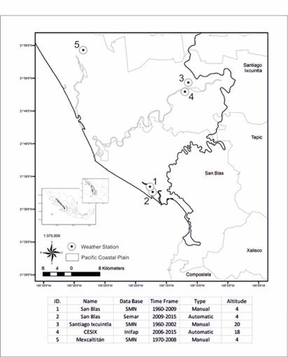
Source: Own elaboration based on cartography or the National Institute of Statistic and Geograph (INEGI, 2000).
Figure 1 Location and characteristics of the weather stations on the case study a fragment of the Pacific Coastal Plain.
According to the description by Nájeraet al. (2020), the prevailing climate is warm sub-humid; mean temperature of 26.2 ºC (thermal oscillation less than 1ºC between the different zones), with an average precipitation of 1334 (rainfall during the summer months of June-September). The hottest months are May and June (35 ºC), and the coldest months are January and February (15 ºC). August is the rainiest month with a 400 mm average. According to the interdecadal analysis of the same authors, the mean and minimum temperatures tended to increase. In contrast, the maximum temperature showed a tendency to decrease, as did precipitation. Temperature anomalies in the area are related between 25 % and 30 % to ENSO and 25 % to PDO; the correlation is higher in the summer months (30 % to 40 % ENSO and 30 % PDO).
The selected area plays a vital role in climate change because it is one of the main reservoirs of the mangrove ecosystem in Nayarit. The mangrove is classified as a sentinel ecosystem against climate effects given its benefits for coastal protection, freshwater maintenance, carbon storage, among others related to biodiversity (Yáñez-Arancibia et al., 2014). These same benefits provide the area with characteristics that have promoted its agricultural, aquaculture, fishing, and tourism uses, which are fundamental for the subsistence of different rural communities in the region (Gonzálezet al., 2009 Nájeraet al., 2021). However, this type of coastal ecosystem has been studied as one of the most vulnerable areas to climate effects because of its geographic location, human-nature subsistence styles, and marginalization (Laraet al., 2008; Ramoset al., 2016).
The climatic data used came from the weather stations available at three institutions. The oldest data series were obtained from the National Meteorological Service (SMN) available through the Climate Computing Project (CLICOM) climatological database. The most recent data series (2010 onwards) were obtained from the National Institute of Agricultural and Livestock Forestry Research (INIFAP) and the Secretariat of the Navy (SEMAR) (Figure 1). We corroborated that each station had at least 80 % consistent data as suggested by other research (Vázquez, 2010; Lobato-Sánchez & Altamirano-del-Carmen, 2017). In order to analyze the variability of at least the last 30 years as recommended by the WMO (Trewin, 2007), the oldest stations (San Blas and Santiago Ixcuintla of the SMN) were joined with the most recent ones (San Blas of SEMAR and CESIX of INIFAP), the homogeneity of their descriptors was corroborated (Nájera et al., 2020). For the case of the Mexcaltitán weather station (SMN), the data series was completed with data estimated by Harris et al. (2014) available in the WorldClim 2.1 database (https://www.worldclim.org) (Fick & Hijmans, 2017). This database was also used to complete the missing data in the rest of the series.
We decided to study the years from 1980 to 2018. For the analysis, the data were grouped into 10-year periods as suggested by WMO (Trewin, 2007) called operational normals. The operational normals facilitate the interpretation of the results. For example, it allows explaining the variability according to the influence of some global signals of natural climate variation, such as the PDO, or other processes of change in the local climate due to anthropogenic actions that are visible over time, such as changes in vegetation cover. In total, we studied three sampling points (San Blas, Santiago Ixcuintla and Mexcaltitán) in four time periods (1980-1989, 1990-1999, 2000-2009, and 2010-2018). The results only can be compared between the dates referred, and by recommendation of the WMO (Trewin, 2007), comparisons cannot be made between different areas.
The statistical validation process was carried out as described in Schuschny&Soto (2009) using the principal component analysis Kaiser-Meyer-Olkin (KMO) test. The principal component analysis is a statistical method that validates the cohesion between information on the same category (indicators within a variable and variables within a dimension). It helps to determine if the indicators selected were necessary to describe the phenomenon studied. The analysis is based on using as few indicators as possible to represent the information's cohesion better. Principal component analysis has become an established technique in climate regionalization because of its ability to capture much of the variation in climate data in a small number of dimensions (Pineda-Martínez et al., 2007).
According to Nardoet al. (2005), three premises must be corroborated before performing the KMO test; the number of observations must be at least three times the number of indicators in the variable, there must be no outlier data, and the data must have a normal distribution. The first premise was met by validating the indicators by variable (four indicators per variable) and each variable in its dimension (two to three variables per dimension), maintaining the 3:1 ratio. The second and third premises were met by standardizing the data using the z-score standardization formula.
The results of the KMO test were interpreted as described in Schuschny & Soto (2009), admitting values above 0.7 as acceptable according to the criteria of Jolliffe (2002). The adequacy of the test was confirmed by performing a hypothesis test with a significance value at a 95 % confidence level. To reduce the number of indicators, we eliminated the indicators that obtained less than 0.8 value in the component. Likewise, we only accepted a percentage of explained variance more significant than 90 % to improve cohesion between variables.
The distances of the indicators were normalized to values 0 to 1 concerning the average to detect the periods different from the normal, allowing us to add the information of the different indicators in the same variable and avoid scale conflicts.
Subsequently, the normalized values of each indicator per variable were summed to obtain subindices from 0 to 1 for each dimension. To obtain the final climate variability index, we sum the subindices of the dimensions normalizing their value from 0 to 1. Finally, the index results were incorporated into a Geographic Information System to represent the climatic variability of the case study cartographically. Given the small number of weather stations, we used Kriging statistical extrapolation (cell size 50), as suggested in the literature, to extrapolate highly variable data with distribution over small flat areas (Sluiter, 2009).
Results
The indicators, variables and dimensions resulting from the statistical validation process are shown in Table 2. As a result of the validation, the number of proposed indicators was reduced from 48 to 24, and the variables were restructured from 12 to six. Four of the five dimensions initially proposed were maintained. The extreme events dimension was excluded according to the KMO value and explained variance obtained (KMO = 0.699, Sig = 0.000, explained variance = 74.4 %). And, one of the two variables of the long-term climate change dimension was excluded because they were similar, and no differences in values were found when we validated the dimension. The final climate variability index application achieved KMO = 0.797, Sig = 0.000 and explained variance of 94.5 %. In the component assembly, dimension 1) climate extreme obtained 0.959, dimension 2) climate anomalies obtained 0.879, dimension 3) natural climate variability teleconnection obtained 0.987, and dimension 4) long-term climate change obtained 0.957.
Table 2 Results of the statistical validation of the indicators, variables and dimensions of the climate variability index from monthly data.
| Dimension | Variable | Indicator | Description | Variable validation | Dimension validation | |
|---|---|---|---|---|---|---|
| 1. Climate extreme | 1.1. Extremes of temperature and precipitation | 1.1.1. Maximum temperature of the monthly highs | Average of the Tmax of the month with the highest annual Tmax of the period. | KMO = 0.867 Sig = 0.000 Explained variance = 94.8 % | 0.977 | |
| 1.1.2. Minimum temperature of monthly minimums | Average of the Tmin of the month with the lowest annual Tmin of the period. | 0.887 | ||||
| 1.1.3. Maximum annual accumulated monthly precipitation | Average of the PP of the month with the highest annual precipitation in the period. | 0.989 | ||||
| 1.1.4. Simple monthly intensity precipitation index | Cumulative annual precipitation divided by the number of months with PP> 1mm. | 0.943 | ||||
| 2. Climate anomalies | 2.1. Temperature and precipitation anomaly index | 2.1.1. Average temperature anomaly index in the period | One minus the mean annual Tp between the mean annual Tp for the period. The result is averaged by the period. | KMO = 0.815 Sig = 0.000 Explained variance = 96.7 % | 0.987 | |
| 2.1.2. Maximum temperature anomaly index in the period | One minus the mean annual Tmax between the mean annual Tmax for the period. The result is averaged by the period.. | 0.962 | ||||
| 2.1.3. Minimum temperature anomaly index in the period | One minus the mean annual Tmin between the mean annual Tmin for the period. The result is averaged by the period. | 0.983 | ||||
| 2.1.4. Accumulated annual mean precipitation anomaly index for the period. | One minus annual accumulated PP between mean annual PP of the period. The result is averaged by the period. | 0.940 | ||||
| 3. Natural climate variability teleconnection | 3.1. MEI teleconnection | 3.1.1. Correlation of mean temperature anomalies with MEI | Correlation of the standardized anomalies of Tp with the MEI index. | KMO = 0.730 Sig = 0.000 Explained variance = 95.8 % | 0.945 | KMO= 0.789 Sig.= 0.000 Explained variance = 98.6 % MEI teleconnection 0.988 ONI teleconnection 0.982 PDO teleconnection 0.988 |
| 3.1.2. Correlation of maximum temperature anomalies with MEI | Correlation of standardized anomalies of Tmax with MEI index. | 0.937 | ||||
| 3.1.3. Correlation of minimum temperature anomalies with MEI | Correlation of standardized Tmin anomalies with MEI index. | 0.987 | ||||
| 3.1.4. Correlation of precipitation anomalies with MEI | Correlation of the standardized anomalies of PP with the MEI index. | 0.964 | ||||
| 3.2. ONI teleconnection | 3.2.1. Correlation of mean temperature anomalies with ONI | Correlation of standardized Tp anomalies with ONI index | KMO = 0.874 Sig = 0.000 Explained variance = 96.8 % | 0.982 | ||
| 3.2.2. Correlation of maximum temperature anomalies with ONI | Correlation of standardized anomalies of Tmax with ONI index. | 0 .943 | ||||
| 3.2.3. Correlation of minimum temperature anomalies with ONI | Correlation of standardized Tmin anomalies with ONI index. | 0.967 | ||||
| 3.2.4. Correlation of precipitation anomalies with ONI | Correlation of the standardized anomalies of PP with the ONI index. | 0.980 | ||||
| 3.3. PDO teleconnection | 3.3.1. Correlation of mean temperature anomalies with PDO | Correlation of standardized Tp anomalies with PDO index. | KMO = 0.842 Sig = 0.000 Explained variance = 96.2 % | 0.970 | ||
| 3.3.2. Correlation of maximum temperature anomalies with PDO | Correlation of standardized anomalies of Tmax with PDO index. | 0.953 | ||||
| Correlation of standardized anomalies of Tmax with PDO index. | Correlation of standardized anomalies of Tmin with PDO index. | 0.963 | ||||
| 3.3.4. Correlation of precipitation anomalies with PDO | Correlation of the standardized anomalies of PP with PDO index.. | 0.964 | ||||
| 4. Long-term climate change | 4.1. Near horizon (2015-2039) A2 RCP 4.5 | 4.1. Mean temperature index of the period compared with HADGEMI | One minus the rate of change between Tp of the period and the Tp estimated in HADGEMI Near horizon (2015-2039) A2 RCP 4.5. | KMO = 0.852 Sig = 0.000 Explained variance = 98.6 % | 0.992 | |
| 4.2. Mean precipitation index of the the period compared to HADGEMI | One minus the rate of change between PP of the period and the PP estimated in HADGEMI Near horizon (2015-2039) A2 RCP 4.5. | 0.982 | ||||
| 4.3. Mean temperature index of the period compared with MPI ECHAM5 | One minus the rate of change between Tp of the period and the Tp estimated in MPI ECHAM5 Near horizon (2015-2039) A2 RCP 4.5. | 0.991 | ||||
| 4.4. Mean precipitation index of the the period compared to MPI ECHAM5 | One minus the rate of change between PP of the period and the PP estimated in MPI ECHAM5 Near horizon (2015-2039) A2 RCP 4.5. | 0.982 | ||||
Following the application of the climate variability index in the case study, the 1980-1989 and 2010-2018 decades were the most variable in the Mexcaltitán weather station area. In the rest of the area, the 2010-2018 decade was the most variable concerning the average (Figure 2).
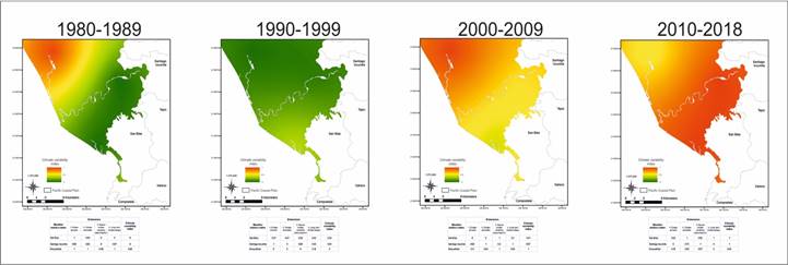
Figure 2 Results of the application of the climate variability index in the case study fragment of the Pacific Coastal Plain.
It should be noted that although the two periods showed high variability, this does not mean that they share the same climatic characteristics. In the case of Mexcaltitán, both periods present antagonistic characteristics. The resulting values for each indicator, in each period and weather station, are shown in Annex 2. (Annex 2)
The climate extreme dimension results showed that the most variable periods were 1980-1989 (San Blas and Mexcaltitán) and 1990-1999 (Santiago Ixcuintla). Based on the oldest period, the maximum monthly temperatures tended to increase in the northern areas (1 to 3 ºC) and decrease in the San Blas area (1 ºC). The same was observed for the minimum temperature of the monthly minimums (decrease of 1ºC in San Blas and increase of 2 to 4ºC in Mexcaltitán). Precipitation decreased in the San Blas and Santiago Ixcuintla zones (between 30 and 50 mm) and increased in the Mexcaltitán zone (50 to 60 mm). The simple monthly intensity index revealed an increase in consecutive months without rain in the San Blas area and a decrease in the Mexcaltitán and Santiago Ixcuintla áreas; however, similarities were observed between the periods 1980-1989 and 2010-2018, so the behavior is possibly related to the influence of PDO.
Regarding the climatic anomalies dimension, the most variable periods were 1980-1989 in the Mexcaltitán area, 2000-2009 in Santiago Ixcuintla and 2010-2018 in the San Blas area. The highest temperature anomalies were in the decrease of minimum temperature; anomalies higher than 4 % and 5 % in San Blas and Santiago Ixcuinlata, and 7 % in Mexcaltitán. In the most variable period, the highest precipitation anomalies were in the average decrease in precipitation; San Blas 10.8%, Santiago Ixcuintla 7.8 %, and Mexcaltitán 7.6 %.
For the dimension of natural climate variability teleconnection, the most variable periods were 2000-2009 and 2010-2018. About ENSO, the highest statistically significant outlier correlations occurred during the 2010-2018 period in all three zones (correlation with temperature anomalies between 15 % and 50 %, and between 15 % and 25 % with precipitation anomalies). About PDO, outlier correlations were observed in 2000-2009 and 2010-2018; in San Blas and Santiago Ixcuintla, unusual negative correlations with temperature anomalies in 2000-2009 and atypical high correlations in 2010-2018, unlike in Mexcaltitán unusual negative correlations with temperature anomalies in 2010-2018 and high correlations in 2000-2009.
Finally, the long-term climate change dimension indicators showed how similar the climate variables are to the climate change scenario models. Values close to zero indicate similarity, while values close to 1 indicate differences. However, in this case, the intention was to highlight those periods different from the average, regardless of the similarities with the climate change models. Thus, the most variable periods were 1980-1989 in the Mexcaltitán area, 2000-2009 in the Santiago Ixcuintla area, and 2010-2018 in San Blas.
Discussion
The proposed climate variability index offers two main strengths; it uses monthly data and was validated by sections. Being an index that uses monthly data, it is a useful option in areas with no daily data reports, and therefore, the application of the WMO climate indices is impossible. Alexander et al. (2019) described this as a recurrent problem in Mexico and Latin America, where most of the available meteorological information comes from daily data collection but is available in monthly compilations to ensure the minimum quality criteria, and the existing quality daily data are complicated to acquire or inaccessible due to their cost. As a sectionally validated index, it can be flexible to be applied in its entirety or by dimensions as required. The validated by sections is an advantage over other indexes; it allows to analyze the causes of climate variability at different time scales, contributing to discuss how global climate change affects the variation in each of them (Amador & Alfaro, 2009). The dimension of correlation with natural climate variability (ENSO and PDO) is an index innovation with respect to others. Natural climate variability is one of the principal causes of local variation in coastal zones (Méndez et al., 2007), and is the scale where have been documented changes in duration and intensity due to global climate change (Méndez et al., 2007; Lobato-Sánchez & Altamirano-del-Carmen, 2017).
On the other hand, three main limitations of the index are discussed: the handling of the data series, operational normals uses, and the validation process. Even though we follow the guidelines from other authors to handling the data, the reconstruction of the series with data from different sources can generate a bias in the results (Vázquez, 2010). Also, the origin of the data may be open to critique (Alexander, 2016); several authors point out that it is necessary to check the status of the SMN weather station network (Luna et al., 2018). About the use of operational normals (analysis in 10-year periods), although it is helpful for the ease to interpret the results, it is also a disadvantage if we desire to know the variation between the years of the periods. According on the average, one period may be more variable than another in the index result, but when we analyze the standard deviation of each of the indicators, it may be that the years of other periods are more variable among themselves. In this regard, we recommend including the standard deviation of the indicators in the results in order to perform complex analyses, keeping in mind that by using operational normals the results only can be contrasted between similar periods (Trewin, 2007). Finally, we suggest repeating the validation process with more observations (preferably complete data series) and more robust statistical methods (Vázquez, 2010).
In addition to the above limitations, it is worth mentioning that there may be other indicators of climate variability that were not included in the dimensions of the proposed index. We use a 2019 review of vulnerability studies in Mexico as a reference in the operative analysis section. The indicators used in the index were extracted from the research cited in that review (and other relevant research cited therein). Although the reference review used a systematized method, there is no guarantee that all existing indicators were taken for each index dimension. For the same reasons, by using indicators derived from vulnerability research, the proposed climate variability index is limited to be used in vulnerability studies or other similar territorial management studies. It should be noted that it is an index designed to evaluate conditions in the present to the past. Even many of the indicators can be estimated in the future through different predictive modeling (dynamic or statistical), it is not recommended that the index be used to evaluate future simulations.
About the results found in the case study, these were consistent with global discussions that affirm variations in temperature extremes accentuated the last 30 years (Alexander et al., 2006; Alexander, 2016). It is also similar to discussions in Mexico; according to Lobato-Sánchez & Altamirano-del-Carmen (2017), there has been a temperature increase in urban areas since 1970 and rural areas since 1980 (of between 1 to 3 ºC in the northwestern region of the country). In general, the most drastic changes between the evaluated periods of the case study were in the Mexcaltitán zone (antagonistic values were obtained in the most variable periods 1980-1989 and 2010-2018), related to the location and the influence of ocean-atmosphere interactions (Nájera et al., 2020). In San Blas and Santiago Ixcuintla, changes were gradual and sustained, with increasing variability over time. The last 20 years were the most variable in these zones, possibly associated with increased urban development and agricultural activities (De la Lanza et al., 2010; Nájera et al., 2020).
Studies have shown that transformations in the biosphere at the micro-scale, especially the reduction of vegetation cover, impact local climate variation (Carvajal & Pabón, 2016). Although it is a debated topic, some authors claim that the formation of patches of anthropogenic land uses (such as agricultural or urban) that differ from the radioactive and thermal properties of the natural vegetation around them, depending on their extension, can produce different thermal gradients. These, in turn, influence mesoscale circulations (10-100 km), causing long-term variations in temperature and precipitation previously unobserved in the regional climate (Baidya & Avissar, 2002). This statement has been verified in different parts of the world (Kouame et al., 2019; Wang et al., 2019; Eiras-Barca et al., 2020; Xian et al., 2020), correlating deforestation and increase in urban and agricultural land cover with historical analyses of climatic variables over 10-year periods. In contrast, natural vegetation would have the opposite effect, creating microclimatic conditions that resist the influence of global climate variability (Pineda-Martínez et al., 2007; Carvajal & Pabón, 2016).
It is speculated that these land use change practices are mainly responsible for the variation in temperature and precipitation patterns in the San Blas and Santiago Ixcuintla area. According to the background described in Nájera et al. (2021), deforestation rates of vegetation cover in the area have been increasing, particularly mangrove annual deforestation rate increased from 0.1 % in 1973-2000 to 1.7 % in 2000-2019. The dates coincide with the decades with the most climate variability. In this sense, local climate variability may be associated with changes in vegetation cover that support microclimates that can deal with the influence of global climate variation and the effects that climate change has on it.
Sustained variations in precipitation and maximum and minimum temperatures of more than one degree with respect to normal (as the last decade turned out in the analysis) can have systemic impacts on ecosystems and human communities. As explained in differents research about coastal zones (Botello et al., 2017), similar to a domino effect, these variations can cause an imbalance in the maintenance of biodiversity that supports essential socioeconomic activities such as fishing and tourism. In addition to the direct impacts of specific hydro-meteorological phenomena such as flooding from torrential rains, hurricanes, and others particular to coastal zones location, such as sea level rise (Ramos et al., 2016). Some of these problems have already been evidenced in the study region (De la Lanza et al., 2010; Gutiérrez, A. et al., 2013; Rodríguez et al., 2017; Lithgow et al., 2019).
While the climate is constantly changing, the problem resides in the speed and magnitude with which it is changing. Climate, derived from large-scale macro-atmospheric and micro-atmospheric interactions related to the biosphere, is susceptible to global climate change and can be mitigated locally by maintaining natural vegetation cover that regulates biogeochemical cycles, such as mangrove cover, estuaries, and flood marshes in the study area. The findings of this research help to rethink the territorial management of the coastal plain, prioritizing the conservation of vegetation covers that face climate change.
We finally suggest analyzing the particular results for each zone, and including as descriptive the indicators that were discarded in the index validation process to have more elements to describe and discuss climate variability. We also suggest using more robust extrapolation methods to analyze the results spatially and corroborate the speculations raised about the relationship between increased climate variability and deforestation.
Conclusions
We obtained a climate variability index validated with the meteorological information available in a fragment of the Pacific Coastal Plain region, delimited by the municipalities of San Blas and Santiago Ixcuintla in the state of Nayarit, Mexico. The definition of the index was based on the indicators used in other studies in the country. As a result, we obtained an index composed of 24 indicators, grouped into six variables and four dimensions; 1) climatic extremes, 2) climatic anomalies, 3) natural climatic variability teleconnection, and 4) long-term climate change. According to the case study analysis, 2000-2009 and 2010-2018 were the most variables periods concerning the average. We expect that the proposed index will be useful for incorporating climate variability in vulnerability assessment and other quantitative studies.

