


 texto em
  Inglês (pdf)
 Artigo em XML
 Referências do artigo
 Enviar este artigo por email
 Citado por SciELO
  Similares em
SciELO
Similares em
SciELO 
 Permalink
Introduction
Forest fires are one of the most important causes of alteration and loss of forest cover; to counteract forest fires it is necessary to implement control and prevention strategies (Thompson, Calkin, Finney, Gebert, & Hand, 2013). However, due to limited resources, the institutions in charge must locate priority attention areas, which can be determined through several criteria. One of those criteria is based on the classification of areas based on forest fire density (Mohammadi, Bavaghar, & Shabanian, 2014), for which there are techniques such as spatial interpolation (Vilar, Martín, & Martínez, 2011) and kernel density estimation (Koutsias, Kalabokidis, & Allgöwer, 2004; Kuter, Usul, & Kuter, 2011). The latter is based on a nonparametric process, whose use involves the selection of a function to estimate the density (Silverman, 1986) and find the appropriate site size to determine it. To do this, a circular site is assumed and an appropriate search area (bandwidth h) is defined (Turlach, 1999); however, when the forest fire density is defined, the statistical criteria that support the selection of the h value are not always clear, even in a visual way (de la Riva, Pérez, Lana, & Koutsias, 2004; Koutsias et al., 2004; Krisp, Peters, Murphy, & Fan, 2009). In this sense, the objective of this study was to establish a statistical process defining the bandwidth h (maximum search area) required for kernel density estimation, in order to develop a replicable and comparable methodology to map priority areas against forest fires.
Materials and methods
Study area
The study was carried out with information from Jalisco, located in the western part of Mexico, where between 17 000 and 20 000 ha are burned annually, with an average of 530 fires (Comisión Nacional Forestal [CONAFOR], 2015). To define the bandwidth (h), georeferenced information was used on the fires that occurred in the period 2005 to 2013 (Figure 1).
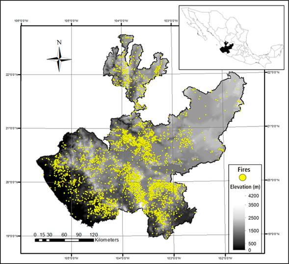
Figure 1 Forest fires occurred in Jalisco in the period 2005-2013 (CONAFOR, 2015). Geographical Coordinate System: GCS_WGS_1984; Datum: WGS84.
Kernel density estimation
Forest fires are georeferenced events that occur differentially in a given region, defining spatial variations in their density (number of fires per unit area) (Salvati & Ferrara, 2015). To map the spatial continuity of this density the following methods are used: 1) classical, which is derived in a) spatial autocorrelation analysis (Anselin, Bera, Florax, & Yoon, 1996), b) cluster analysis (point clustering) (Kulldorff & Nagarwalla, 1995) and c) spatial autoregression models (Anselin et al., 1996); and 2) density maps, where the techniques of quadrant analysis and kernel density are used (Fuenzalida, Cobs, & Guerrero, 2013). The latter has been used when historical fire data is available (Koutsias et al., 2004, Kuter et al., 2011). Kernel density is a non-parametric technique based on several functions, some of these are: the square function (Silverman, 1986), the uniform function, the Epanechnikov function, normal distribution, triangular function and quartic function (Turlach, 1999). In this way, the kernel density estimator, for a multivariate case, is defined based on the following mathematical expression (Amatulli, Perez-Cabello, & de la Riva, 2007):
where,
n |
number of observation points |
h |
bandwidth |
K |
central module (kernel) |
x |
vector of coordinates representing the location where the function is estimated |
X |
vectors of coordinates representing each observation point |
d |
number of dimensions in space. |
Based on the above, kernel density estimation helps to generate continuous surfaces of forest fire density. For that purpose, local neighborhood calculations are used under the structure of a grid (grid of cells), where the density value, at a given point or cell, results from an estimate based on the values of several points around it; nearby values have greater influence, while distant ones have less weight in the estimate. This conforms to the first law of geography, which states that everything is related to everything, but things that are close are more related to each other than things that are more distant; however, this process is limited to a certain distance, which is defined by establishing a bandwidth (h) (de Smith, Goodchild, & Longley, 2009).
Determining bandwidth (h)
Because the application of the kernel function requires that a bandwidth (h) be specified, this study considers the processes described below.
1) Theoretical polygon. It is assumed a theoretical square surface, where the theoretical h is defined based on the length of the corresponding theoretical area (de la Riva et al., 2004):
2) Mean random distance (MRD). The criteria used to define the MRD were expressed mathematically in the following way (de la Riva et al., 2004):
3) Average distance of the nearest neighbor. The h value is defined by estimating the average distance among nearest neighbor fires (Koutsias et al., 2014).
4) Silverman's rule of thumb. It considers a non-Gaussian kernel function, where the h value is defined as follows (Silverman, 1986):
In other cases, for example with a triangular kernel function, the h value would be estimated with the following equation:
5) Interquartile range. It assume that distribution deviates from normality and use the following algorithm to determine the value of h (Vrahimis, 2010):
Validation criteria
The statistically most adequate h value was selected by the following criteria.
1) Root mean square error (RMSE). This statistic was determined in terms of the difference between estimated density and true density, where the lowest RMSE was selected. First, we calculated the mean squared error (MSE) that incorporates both the variance of the estimator and its bias and, later, the square root of MSE was obtained:
Based on this, 1 000 random points were located in the study area to determine RMSE; and with them two common surfaces (circular area) were compared: 10 and 100 km2. The real value of the number of fires from 2005-2013 and the estimated value of the number of fires defined by the kernel function were determined in these areas.
2) Root mean integrated squared error. The comparison was made under the same criteria indicated for the RMSE. For this, the mean integrated squared error (MISE) was estimated and then the square root (RMISE) was calculated, from the equation proposed by Seaman and Powell (1996):
3) Coefficient of variation (CV). Taking into account that the size of h defines a sampling unit allowing to capture the variability of the number of forest fires, several circular surfaces or reference sites (CRS) were analyzed in the study area: 1, 2, 4, 8, 10, 15, 30, 50, 70, 100, 150 and 200 km². In addition, the following sampling intensities completely randomly distributed were evaluated: 100, 300, 500 and 1000 SIR. The contained fires in each SIR were counted and, then, the CV defined in relation to the 12 sizes of SIR was plotted; in this way, the surface of SIR and its corresponding h were selected at the point where the variability trend starts an asymptotic behavior.
4) Comparative percentage. Similar to the CV, the increase in h eventually defines an asymptotic behavior of RMISE, so, an objective selection of h is to locate the break point or at least a break rank, where this behavior starts. For this, the percentage representing the value of RMISE was estimated in relation to the immediate superior value, which was called comparative percentage (CP), which is calculated with the following equation:
Results and discussion
Estimating h
Table 1 shows the bandwidth estimates (h = search area), resulting from the processes analyzed. There is great variation in the h values obtained; the range between the maximum and the minimum value was 39 356.34 m with an average of 10 936.74 ± 9 955.04 m. Table 1 also shows the values of the criteria on which the analyzed processes are based. It is important to note that some of the criteria are particular to certain processes, so they were not used in all cases.
Table 1 Bandwidth (h) estimation corresponding to the kernel density estimator, according to different processes.
| Process | Source | H (m) | P (km2) | A (km2) | N | Particular criteria |
|---|---|---|---|---|---|---|
| Theoretical polygon | de la Riva et al. (2004) | 2 550 | 20 | 13 | Side = 3 605.55 m D = 5 099.02 m | |
| Mean random distance | de la Riva et al. (2004) | 3 472 | 38 | 5 | 0.52 | A = 25, 100, 225 and 400 km2 |
| 5 395 | 91 | 10 | 0.86 | |||
| 6 750 | 143 | 15 | 1.23 | |||
| 7 797 | 191 | 20 | 1.65 | |||
| Twice the mean random distance | Kuter et al. (2011) | 6 944 | 151 | 5 | 0.52 | A = 25, 100, 225 and 400 km2 |
| 10 790 | 366 | 10 | 0.86 | |||
| 13 500 | 573 | 15 | 1.23 | |||
| 15 594 | 764 | 20 | 1.65 | |||
| Average distance to nearest fire | Koutsias et al. (2004) | 4 980 | 78 | |||
| Silverman's Golden Rule | Silverman (1986) | 9 051 | 257 | Factor = 1.06 DS = 46 562 n = 4 821 | ||
| Triangular kernel function | Turlach (1999) | 21 996 | 1 520 | Factor =2.576 DS = 46 562 n = 4 821 | ||
| Interquartile range | Vrahimis (2010) | 41 906 | 5 517 | IQR = 64 824 IQR/1.34 = 48 376 DS = 46 562 n = 4 821 |
h = search area, DS = standard deviation of the sampled points, A = average polygon size, D = diagonal (m), N = average number of forest fires, n = number of sampled points, P = size of the sampling polygon (km2), IQR = interquartile range.
In the process of the theoretical polygon, the selection of h is according to the scale on which the information is held; that is, if the information is presented in pixels of 10 x 10 km, then a theoretical area is established corresponding to half the length of the frame defining the pixels (de la Riva et al., 2004). However, although this alternative may be practical, it is not based on statistics; for example, it should be considered that the variance of the number of fires can change if one works with different areas defined by multiples or submultiples of pixel size. As an alternative, it was proposed to base the definition of h on the average size of polygons, assuming a polygon of 20 km2 as the theoretical square surface, where the theoretical h (2 550 m) was defined based on the length of the corresponding theoretical area (de la Riva et al., 2004), which resulted in the lowest h value of all the processes analyzed.
On the other hand, the average distance defined among 1 000 points located randomly (MRD), was used as h value, which can be shown from two perspectives (Kuter et al., 2011): a) local, regarding the average polygon size and a number of ignition points per polygon, and b) global, where the total size of the study area and the total number of ignition points are considered. In this case, the first perspective was considered, since it allowed to establish the value of h in relation to the different sizes of polygons that were analyzed (25, 100, 225 and 400 km2); however, the differences among the corresponding h values were not so considerable, with values of 3 472, 5 395, 6 750 and 7 797 m, respectively. Therefore, based on that recommended by de la Riva et al. (2004), twice the mean random distance was also analyzed as the h value; however, neither the MRD nor its double version work directly with the points defining the location of forest fires.
To understand the problematic of the selection of h, it must be understood that it is a variable (within a mathematical model) that can be defined in fixed or adaptive mode. Regarding the first option, h was also defined based on the concept of neighbor's average distance, where the nearest fire point was taken (Koutsias et al., 2004). In this way, the resulting value was lower than the average of MRD defined (5 854).
One of the first approaches to a selection criteria of the h value is based on the “Golden rule of Silverman”, which assumes a kernel function with a Gaussian base, to approximate univariate data, where it is suggested to select the h value minimizing the mean integrated squared error (risk function) (Turlach, 1999). In this study, the h value resulting from this perspective was 9 051 m, which approaches to the criteria average of twice the MRD analyzed (11 707); however, regarding a triangular kernel function, the value of the resulting h was more than double (21 996).
On the other hand, considering that the distribution deviates from normality, the implementation of the interquartile range algorithm (Silverman, 1986) resulted in an extremely overestimated h value. This coincides with that found by Silverman (1986) in a case of a bimodal distribution with separate means, defining a highly skewed distribution.
Continuous surfaces
Once the h values were defined, the kernel function estimator was implemented, defining two options for the generation of continuous surfaces: a) based on the estimated density probabilities; and b) based on the estimate of the corresponding density (number of fires per unit area). Taking into account that in the definition of fire management strategies it is necessary to have mapping to locate and size priority areas, the continuous surfaces were generated based on the density estimated with the different h values. Figure 2 shows the continuous surfaces, observing that the surface "softens" as the value of h increases, while, at low h values, the continuous surface tends to define circular regions around the points (forest fires), what is known as the “bull's eye” phenomenon.

Selecting bandwidth (h)
An option for selecting the h value is to do it intuitively, based on a visual perspective (de la Riva et al., 2004; Koutsias et al., 2004; Krisp et al., 2009); that is, subjectively selecting the h value producing a continuous surface, whose softness is more “random” than “structural” (Kuter et al., 2011). Therefore, it is considered that this selection is an act of art rather than science (Krisp et al., 2009), which does not allow to define replicable processes and will always be subject to the experience of the person making such selection (Turlach, 1999). As an alternative, this study implemented statistical criteria, seeing in Figure 3 that when comparing continuous surfaces (generated by the different h values), errors tend to increase as the h value increases. This trend is adjusted to a second-order polynomial regression (Table 2), without defining an asymptotic behavior, so it is not possible to establish a breakpoint that allows defining a maximum h value (or a range). This suggested that a common comparison area should be established to analyze forest fire density estimations.
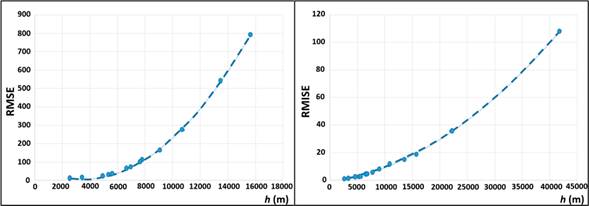
Figure 3 Error distribution in relation to bandwidth (h), when comparing forest fire density estimations in areas defined by different h. RMSE = root mean square error, RMISE = root mean integrated squared error.
According to the above, regarding the RMSE and a common comparison surface of 10 km2, Figure 4 shows that when the h value increases, the estimation error also increases, and as it was observed in Figure 2, the "smoothing" of the continuous surfaces increases in proportion to the increase in the h value. This implies that the selection of a smoothed continuous surface (de la Riva et al., 2004; Koutsias et al., 2004; Kuter et al., 2011) does not necessarily define the best h value. Table 2 shows the statistics corresponding to this trend. Whereas the utility of the RMSE formula can be doubtful in practice, since it depends on the f unknown density, the RMISE was used as a global measure of the estimator's precision (Álvarez & Yohai, 2012). The trend between RMISE and h was similar; however, the adjustment model had a lower r2 value (Table 2), showing an asymptotic behavior when h = 15 000 m.
Table 2 Trend models between the relationship of statistical selection criteria and bandwidth value (h).
| Comparative | Criteria | Model | r2 |
|---|---|---|---|
| 10 km2 | RMSE | = 0.3638ln(h) - 2.2248 | 0.9452 |
| RMISE | = 0.0465ln(h) - 0.1052 | 0.7823 | |
| 100 km2 | RMSE | = 0.7927ln(h) + 5.1792 | 0.8135 |
| RMISE | = 0.1977ln(h) + 0.4507 | 0.4437 | |
| h | RMSE | = 5E-06h 2 - 0.0381h + 75.0210 | 0.9992 |
| RMISE | = 5E-08h 2 + 0.0006h - 1.7225 | 0.9999 |
RMSE = root mean square error; RMISE= root mean integrated squared error.
In the case of the common area of 100 km2, the errors of RMSE were greater and very similar among the different h values. This trend suggests that, as the area of comparison increases, the error of the estimates tends to be more homogeneous. Regarding the RMISE, the behavior was similar to that of RMSE; nevertheless, it is observed that, in low h values, there is a marked tendency to reduce the error. On the other hand, in both cases (RMSE and RMISE) an asymptotic tendency is defined from h values lower than 5 000 m. The comparison of RMISE, regarding the areas of 10 and 100 km2, suggests that the h value, with constant behavior of the error, is between 5 000 and 10 000 m, where the values defined in the processes are shown in Table 1: mean random distance (h = 5 395, 6 750, 7 797 m), twice the mean random distance (h = 6 944 m), average distance to the nearest fire and “Silverman's golden rule” (Silverman, 1986).
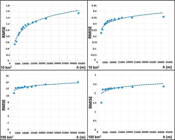
Figure 4 Estimation error distribution of forest fire density in relation to bandwidth (h), regarding two comparison areas. RMSE = root mean square error; RMISE = root mean integrated squared error.
According to the results, the size of h with the lowest estimation error (RMISE) should be chosen, which corresponds to the lowest h value. However, this does not guarantee that we have the most adequate h value, since it should also be considered that the variation (CV) of forest fire density decreases as the size of h increases (Figure 5). However, the choice of low CV values does not guarantee the choice of the most suitable h value.
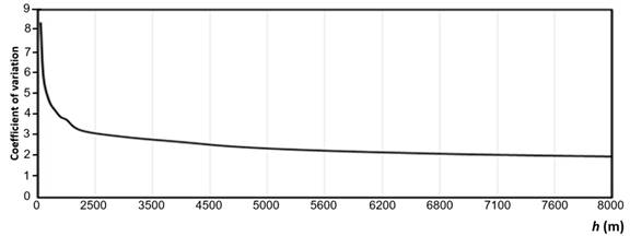
Figure 5 Coefficient of variation trend of forest fire density in relation to the increase in bandwidth (h).
Based on the above, it was found that variance (CV) decreases when h value increases, while the bias (RMISE) increases; the opposite occurs when h value decreases. Therefore, the definition of the most adequate h value will be that which represents a compromise between variance and bias (Álvarez & Yohai, 2012). For this, based on the asymptotic behavior of RMISE, an alternative way is defined to determine the h value, by locating the break point or at least a break rank where the asymptote starts. For this purpose, the comparative percentage (CP) values were determined, where a break range is defined, around 5 000 and 6 000 m (Figure 6 a) , this situation coincides for the two polygon sizes of comparison (10 and 100 km2). In order to locate a breaking point, the CP trends were modeled (P-10: y = -9E-08x2 + 0.0025x + 83.87, [R² = 0.5891]; P-100: y = -1E-07x2 + 0.0035x + 79.358, [R² = 0.5891]), whose crossing defined a point of coincidence around 5 600 m (h), which is within the breaking range defined (Figure 6 b). Finally, the statistically most adequate h value will be the one that comes closest to 5 600 m and which is within the range of 5 000 and 6 000 m. According to this, the definition process of h that is closest to this value is the mean random distance (h = 5 395 m).

Conclusions
It is possible to establish a statistical process of bandwidth (h) selection, for kernel density estimation of forest fires. In this way, we tend to define processes and results, which can be replicable, comparable and compatible, which are not conditioned to the participation of experts, which avoids the use of subjective criteria such as the visual appreciation of continuous surfaces, defining the spatial variation of forest fire density. There was great variation among bandwidth values, which implies that there is no single and universal process for all cases. This is because kernel density estimation are conditioned to several factors, such as spatial resolution of information (cell size), bandwidth, number of points to be considered and intrinsic characteristics of the phenomenon under study.

