


 nova página do texto(beta)
 Inglês (pdf)
 Artigo em XML
 Referências do artigo
 Enviar este artigo por email
 Citado por SciELO
  Similares em
SciELO
Similares em
SciELO 
 Permalink
Introduction
The 2013 Mexican Energy Reform was implemented to liberate the energy sector, allowing new participants to enter the electrical industry in the generation, transmission, distribution, and commercialization of electricity. The liberation process will encourage a competitive environment since new participants will seek to generate electricity at the lowest cost, for which they will make investments focused on modernizing the infrastructure and implementing automated processes, thereby seeking to achieve an increase in operating efficiency. The electricity reform is expected to improve the electrical service offered, as mentioned in Article 4 of the Electricity Industry Law (Diario Oficial de la Federación, 2014) "significant benefits in efficiency, quality, reliability, continuity, safety, and sustainability," as well as lower electricity prices for industrial, commercial, and residential consumers.
These benefits must be transferred to the final consumer as welfare increase. In this sense, Ramírez et al. (2021) developed a study to measure the Mexican population's welfare improvement of those energy goods consumers related to Mexico's energy reform; the study is focused on electricity, liquified petroleum gas (LPG), and gasoline for the period between 2010 and 2018. Ramírez et al. (2021) analysis concluded that after Mexico's energy reform, electricity, liquified petroleum gas (LPG), and gasoline consumers have experienced welfare gains compared to consumers in the 2010-2014 period. Unfortunately, it was also found that welfare gains are associated with enormous amounts of resources dedicated to subsidizing energy goods. Finally, Ramírez et al. (2021) mention that efforts must focus on increasing efficiency through the energy supply chain rather than subsidies to achieve sustainable welfare gains.
Article 94 of the Electricity Industry Law states that: "National Center of Energy Control (CENACE) will operate the Wholesale Electricity Market” following this Law. The Short-Term Energy Market is part of the Wholesale Electricity Market that comprises three sub-markets: Baja California Interconnected System (BCA), South Baja California Interconnected System (BCS), and National Interconnected System (SIN).
The Short-Term Energy Market operates based on an economic dispatch process described in the General Provisions of the Short-Term Energy Market of the Electricity Market Rules (2015). Rule 9.1.8 provides the process for assigning hourly electricity price for each network connectivity node with physical delivery and energy withdrawal (NodeP), which is considered equal to the marginal cost of its generation, determined by the variable cost at which the last megawatt-hour was dispatched. This marginal cost of supply is called Local Marginal Price (LMP). By applying CENACE’s economic dispatch algorithm, the LMP is calculated for each of the NodePs of the Day-ahead market (MDA) and Real-time market (MTR); the price estimation result will have three marginal components: energy, losses, and congestion.
It is essential to keep in mind that the demand for electricity depends on factors related to the weather, such as temperature, rainfall, wind speed, etc., and daily consumption regarding market intensity and consumer activities during weekdays, weekends, holidays, etc. It is worth mentioning that seasonality is one of the main characteristics that make price dynamics behave differently concerning other financial assets, since it presents daily, weekly, monthly, and annual levels. These characteristics, described by Weron (2014), cause LMP volatility dynamics, which can produce significant differences between the projected price and the trading price in the short-term market, leading to substantial financial losses for the market participants who do not have adequate financial hedging. Electricity price volatility can be twice as high in magnitude as that of another commodity or any financial asset, as described by Weron (2014), which represents a source of risk if a proper hedging price volatility strategy is not in place.
Due to the price dynamics described above, electricity price series behavior analysis is of utmost importance to have solid quantitative elements that facilitate making estimations with reasonable levels of accuracy, with which hedging products can be designed in the event of an extreme change in the LMP. It is also important to have a robust risk management strategy, to achieve financial results within the defined margins, and avoid severe economic losses in a market in which generation costs and sales prices are highly volatile, such as the electricity market. By implementing this practice, market participants and consumers have electricity price certainty, ensuring better financial planning, which is essential for any productive economy sector in terms of efficiency, productivity, and financial stability.
Although competitive electricity prices benefit the productive sectors in terms of efficiency and productivity, there will not always be evidence of a causal relationship between electricity production (EP) and Gross Domestic Product (GDP). In this sense, Massa and Rosellón (2020) prepared a study for the case of Mexico for the period 1965-2018 to identify the Granger causality directions between EP and GDP. Their results suggested a neutral effect, which led them to the conclusion that policy implementation focused on EP improvement may not have any impact (positive or negative) on the GDP. They also concluded that neutrality should be considered as an opportunity because a secondary Electricity Reform objective is related to the energy transition which aims to achieve 50% of electricity generation with clean energies, especially solar and wind, by 2050. They state that the energy transition would not have any effect on economic performance and would also be an opportunity to develop a national competitive electric power sector that relies less on US electricity imports. Sarmiento et al. (2021) mention that achieving the 50-50% generation goal, has already implied fast short-run developments of natural gas and renewable infrastructure in Mexico, such as investments to increase the pipeline systems and solar and wind auctions.
According to Energy Generated by Technology Type (2021), clean electricity generation (wind and solar) represents 11%, while combined-cycle plants represent 59% of electricity generated by July 2021. From this statistic it can be assumed that the Mexican electricity industry relies on coal, diesel, fuel oil, and natural gas for electricity generation through combined-cycle plants. In this sense, Sarmiento et al. (2021) state the crucial role of natural gas in the energy systems of Mexico and the United States. They analyzed the impact of different natural gas prices on the power generation matrix across both nations, showing an explicit dependency of Mexican electricity generation on natural gas, wind, and solar technologies. Their study mentions that market liberalization reforms have increased reliance on U.S. shale gas based on economic arguments of liberalization, competition, and cost minimization. The study also states that importing shale gas from the U.S. represents an economic solution to meet Mexico's growing natural gas demand and is linked to the development of combined-cycle power generation.
From the perspective of hedging electricity price volatility, events that cause market and electricity price disruptions should be considered. One of the most disruptive events in modern history is the current case of the economic crisis related to the pandemic caused by the SARS-COV-2 virus, which has forced people to change their habits, resulting in socioeconomic changes, due to the sanitary restrictions and lockdowns that have been implemented globally. In this sense, Corpus-Mendoza et al. (2021) evaluated the impact of the pandemic on urban mobility, electricity consumption, and
This analysis proposes a methodology for hedging and forecasting electricity prices, focusing on applying the STL decomposition model for seasonal adjustment following the utilization of NIG distribution to obtain NIG parameters from empirical series to generate a NIG simulated series, and finally verifying simulated series fitted to NIG distribution empirical parameters through the application of goodness-of-fit tests. Since it is known that the logarithmic returns of financial prices do not fit the Normal distribution, the aim is to demonstrate that LMP returns can be modeled as a financial asset using the NIG distribution to achieve a better fit compared to the Normal distribution when performing a numerical hedging valuation that has LMP returns as an underlying asset.
The present analysis has two main contributions. First, we propose utilizing the LMP Marginal Energy Component as the underlying asset for hedging price volatility, since said component is the same for all NodePs belonging to the same electrical system; we also develop a detailed description of the reference node selection criteria for each electricity market, as well as a description of LMP components. Second, we propose the first methodology for hedging electricity price volatility for the Mexican Electricity Markets, considering for this analysis two time periods, the population of data that includes the pandemic period and the period related to the pandemic. Empirical results obtained indicate that the price dynamics of electricity can be captured and simulated through this methodology for every economic situation, even for periods of economic crisis.
This analysis is organized as follows: In Section 1, the literature review is carried out on the techniques used to model electricity price series and electricity derivatives valuation, and a review of heavy-tailed distributions that can improve financial asset series is performed. Section 2 describes the data series selection criteria for the present study, while the data series are described in Section 3. In Section 4, the STL decomposition model is described. Section 5 develops the methodology used to demonstrate that the deseasonalized LMP energy component logarithmic returns fit NIG distribution, and finally we present the conclusions of the analysis.
I. Literature review
Janczura and Weron (2013) mention that to model electricity price series, their particular characteristics are related to seasonality at the annual, monthly, weekly, and daily levels, while mean reversion and spikes in prices must also be taken into consideration. According to Weron (2014), seasonality is one of the main characteristics that make price dynamics behave differently from other financial assets, since it presents daily, weekly, and annual levels. Cleveland et al. (1990) developed the STL model of seasonal and trend decomposition based on LOESS; the model is a filtering procedure to decompose a time series into its trend, seasonal, and remainder components. The model was developed mainly to have a decomposition process, which could be implemented computationally. The main characteristics of this model include the flexibility to specify the amount of variation in the trend and seasonal components and that it provides the capacity to specify the number of observations per cycle of the seasonal component, obtaining robust trend and seasonal components that are not distorted by the transient aberrant behaviors of the data, which are relevant for the present analysis. Sun et al. (2019) used Seasonal and Trend decomposition by LOESS decomposition (STL) to forecast monthly electricity sales, by decomposing the electricity sales series into their seasonal, trend, and remainder components, carrying out the analysis of each component independently, trying to identify the factors that influence each component and then integrate again an adjusted series with which it is possible to make reliable sales forecasts.
The development of valuation models for electricity derivatives has been treated from the perspective of financial mathematics and econometrics. Vehviläinen (2002) stated that modeling the electricity spot price process utilizing Black and Scholes's model assuming Geometric Brownian Movement is not recommended for the electricity market. His analysis proposes a mathematical model attached to traditional financial theory, where he describes that since electricity is not an asset that can be stored, it must be modeled differently compared to other commodities. As electricity is consumed when it is generated, the spot price also depends significantly on the system's stability, since a failure in a network component can cause unexpected jumps, spikes, and high price volatility.
Brager et al. (2010) present a model that considers jumps and spikes, which can be calibrated for the price series once both parameters are a function of time. They mention that since electricity cannot be stored (at an acceptable cost), there is no formula to estimate "cost-of-carry," so there is no specific relationship between the spot price and the future price, explaining that the expected spot price is directly influenced by supply and demand in the future. Expected demand is influenced by weather forecasts, business cycles, customer behavior, etc. Moreover, the expected supply depends on the futures of other commodities used for electricity generation, such as oil, gas, and coal, which cause high volatility in future prices.
From an econometric perspective, Chan et al. (2008) comment on developing a model that can accurately capture the underlying asset's characteristics, especially the number and intensity of the asset jumps that occur. Chan et al. (2008) mention that, continuing with the seminal work of Johnson and Barz (1999), various studies have been carried out where the jump-diffusion model commonly used in asset prices and interest rates has been adopted to model electricity prices, Escribano et al. (2011), Geman and Roncoroni (2006), to name a few.
Chan et al. (2008) also consider the work of Andersen et al. (2007) which describes the jump-diffusion model as a combination of two components, first, a smooth continuous sample path process and, second, a discontinuous component of the jump process. Chan et al. (2008) state that although the reference framework of a jump-diffusion process is intuitive theoretically, its econometric implementation has some relevant shortcomings. Chan et al. (2008) remark on the difficulty in identifying the jump components and the smoothing variations process in the price, since the results obtained using jump-diffusion models do not allow the identification of these components. Chan et al. (2008) also mention the work carried out by Jiang (1999), which states that conditional volatility, the size of the spikes, and frequency are not observable variables, so they must be estimated as dynamic variables, making it challenging to identify a diffusion model with jumps capturing the characteristics of the underlying price.
As has been mentioned, mathematical and econometric models have some limitations in capturing the characteristics of electricity prices, especially concerning the magnitude and frequency of observed jumps and spikes. These shortcomings have generated the motivation to analyze the behavior of the underlying asset by fitting a distribution, in the case of electricity prices, the NIG distribution may capture the dynamics of jumps and spikes since it is a heavy-tailed distribution, which can be used to carry out the valuation of electricity options or futures numerically and for electricity price forecasting.
Given this context and the difficulty of having a general differential equation for any class of financial asset, a group of researchers has taken an approach that encompasses applying different families of probability distributions. In particular, the Generalized Hyperbolic family has proven to be an ideal choice given the presence of heavy tails.
The Generalized Hyperbolic family proposed by Barndorff-Nielsen (1977) is specified by five parameters, one of them "λ". If this parameter is set to -0.5, Normal-Inverse Gaussian (NIG) is obtained. Barndorff-Nielsen (1995) also used NIG distribution to model observations with heavy tails.
It is essential to mention that the Generalized Hyperbolic family not only fits financial asset returns such as the IPC and S&P 500 indices, as stated by Trejo et al. (2006), but is also capable of fitting cryptocurrency returns. On this particular point, Núñez et al. (2019) point out the ability of the NIG distribution to fit Bitcoin's returns concerning seven of the leading global currencies for periods with explosive behavior and subsequent collapse (financial bubble). In addition, NIG distribution can model and fit the indices of Brazil, Russia, India, and China (BRIC) for different periods and even during economic recessions and crises, as demonstrated by (Núñez et al. 2018).
II. Methodology Description
The following section describes the models and techniques used to develop the proposed methodology to capture the behavior of the LMP Marginal Energy Component.
Logarithmic Returns Estimation
Logarithmic returns were obtained as follows:
Data Series Unit Root Test
The Augmented Dickey-Fuller is applied to verify that the data series first difference is stationary as defined by Dickey and Fuller (1979):
LMP Return Data Series Modeling Using STL Decomposition
The STL Decomposition Model developed by Cleveland et al. (1990) was applied. The model is a filtering procedure for performing the decomposition of a time series into its trend, seasonal, and remainder components, which is denoted as follows:
Where:
The following criteria, described by Cleveland et al. (1990), justify the selection of the STL decomposition model to perform the seasonal adjustment of Electricity Price Returns (EPR): “Flexibility to specify the variation amounts in trend and seasonal components provides the capacity to specify the number of observations per cycle of the seasonal component to any integer greater than 1, and robust trend and seasonal components that are not distorted by transient, aberrant behavior in the data are obtained”.
Analysis of STL Decomposition Parameter Selection
The following section describes parameter values used to perform the seasonal adjustment of EPR, according to Cleveland et al. (1990).
The seasonal component
Parameter
Parameter
Parameter
The Trend Smoothing Parameter
Obtaining Deseasonalized Data Series
According to Cleveland et al. (1990), the STL decomposition model is based on an additive procedure, establishing that the original series is the arithmetic sum of the seasonal, trend, and remainder components, as shown in equation (3).
Starting from this statement, we can take advantage of this property to subtract the seasonal component from the original data series and eliminate the seasonality component and thus the Deseasonalized Energy Price Returns (DEPR) series that is a stationary series without seasonality:
Where
Methodology for Adjusting NIG Distribution to Deseasonalized Returns
To fit the NIG distribution to the DEPR, obtained in the section above, the methodology proposed by Núñez et al. (2018) was applied as follows.
Descriptive statistics
Descriptive statistics estimations of DEPR are performed to determine the mean, variance, skewness, and kurtosis values empirically. In this case, the data series distribution is not expected to fit the Normal distribution.
Normality tests
Normality tests are used to determine whether the data series fits the Normal distribution. If not, NIG distribution would be an ideal candidate and can be used to adjust the DEPR. The following Normality Tests are considered as part of the methodology: Anderson and Darling (1954) “Anderson-Darling”, Pettitt (1976) “Cramer-von Mises”, Jarque and Bera (1980) “Jarque-Bera”, Lilliefors (1967) “Lilliefors”, and Shapiro and France (1972) “Shapiro-France”.
Obtaining NIG distribution parameters by MLE
Barndorff-Nielsen (1997) presented The Normal Inverse Gaussian (NIG) distribution, as a variance-mean mixture distribution, to construct stochastic processes for statistical modeling purposes, such as turbulence and finance; its density function is defined as follows:
Where:
And:
Where
NIG parameters were estimated from each of the DLMPR by Maximum Likelihood Estimation (MLE).
Simulating NIG distributed data series
Data series simulation was performed using numerical NIG distribution simulations with the parameters obtained from each of the empirical DEPR considered into the analysis. Each simulated series was created considering the same number of observations as the original series.
Goodness-of-Fit Tests
Goodness-of-fit tests were used to determine the similarities between the empirical and NIG simulated DEPR distribution and obtain conclusive statistical elements to demonstrate that the empirical series can be fit into the NIG distribution. The Anderson and Darling (Stephens,1979) “Anderson-Darling”, Massey (1951) “Kolmogorov-Smirnov”, and Kruskal and Wallis (1952) “Kruskal-Wallis” goodness-of-fit tests were estimated.
III. Data Description
Reference Node and Marginal Energy Component
The Short-Term Energy Market Manual establishes in base 4.4.8 that: "For each hour of the operating day, the Local Marginal Price components depend on the selection of a reference node in each interconnected system”. Table 1 shows the Reference Nodes for LMP estimation (2021) chosen by CENACE for each interconnected system.
Table 1 Reference Nodes for the LMP estimation
| Interconnected system | Reference Node | ||||
| Node Code | Name | Voltage Level |
Charging Zone |
Regional Control Center |
|
| National (SIN) | 03QRP-400 | Querétaro Potencia | 400 | Querétaro | Occidental |
| Baja California (BCA) | 07PJZ-230 | Presidente Juárez | 230 | Tijuana | Baja California |
| Baja California Sur (BCS) |
07OLA-230 | Olas Altas | 230 | La Paz | Baja California Sur |
Source: Reference Nodes CENACE.
The criteria used to select the reference node for each interconnected system are mentioned below, according to CENACE:
The node was selected since it is located in the center of the system, for numerical stability reasons.
It was intended to be a substation with high reliability and a voltage level greater than or equal to 230 kV.
There must be no load or generation at the node and, therefore, there will be no settlement for any market participant and LMP will not be estimated for reference nodes.
As previously mentioned, "the components of the LMP depend on the selection of a reference node in each interconnected system". Hence, a series of parameters are defined in the Physical Network Model and the Commercial Market Model to estimate the LMP components for each of the interconnected system nodes. However, the information of the reference node parameters is classified and reserved for market participants and trusted external users. Nevertheless, it is known that (i) the marginal energy component of the LMP is the same for all NodePs in the same interconnected system, for each hour of the day of operation, and that (ii) the marginal component of losses and congestion in the reference node is equal to zero for the reference node. With these statements it can be concluded that the LMP Marginal Energy Component (ECP) of any NodeP would be equivalent to the Reference Node Price Series (RNP) within each interconnected system. Thus, the ECP can be selected to perform the hedging valuation methodology.
Data Selection
For this statistical analysis, the ECP of a NodeP for each of the three interconnected systems were used. To maintain consistency with the name and code of the reference node assigned by CENACE, the NodePs selected are those placed in the same location as the Reference Node of each of the interconnected system. Some NodeP and reference node code similarities can be observed due to this selection criteria. It is important to mention that the reason for choosing the ECP is because, as described above, it is equivalent to the RNP. It should be mentioned that the Reference Nodes are not considered NodePs and therefore do not exist within the CENACE NodeP catalogue. However, there is a NodeP within the catalogue with the same name as the Reference Node but different characteristics. Table 2 shows the names and codes of the NodePs from which the EP was obtained.
Table 2 ECP NodePs
| System | Charging Zone | Name | NodeP | Reference Node |
| SIN | Querétaro | Querétaro Potencia | 03QRP-115 | 03QRP-400 |
| BCA | Tijuana | Presidente Juárez | 07PJZ-115 | 07PJZ-230 |
| BCS | La Paz | Olas Altas | 07OLA-115 | 07OLA-230 |
Source: Own estimations with information from the CENACE "NodeP Catalogue and reference nodes."
ECP empirical observation frequency is on an hourly basis, seven days a week. For the present analysis, two scenarios are considered. The first scenario analyzes the ECP of each of the interconnected systems considering the entire population of data up to 09/07/2021. The second scenario examines the ECP of each of the interconnected systems for the period corresponding to the SARS-COV-2 pandemic between 01/04/2020, the day when the health contingency was established, and 09/07/2021. Figure 1 shows the ECP graphic for each scenario considered; all the observations shown in the graphics correspond to data population, and the sample in red corresponds to the SARS-COV-2 health contingency period.
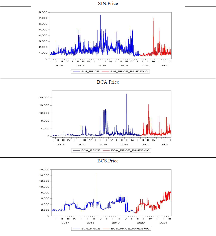
Note: (Blue) and (Red) series corresponds to data population, (Red) series corresponds to the SARS-COV-2 health contingency.
Source: Own estimations with information from CENACE.
Figure 1 ECP Data Series Scenarios
The Maximum Daily LMP Marginal Energy Component Data Series (MECP) was obtained from the hourly-basis series of the ECP. It was assumed that the MECP could be the price of the underlying asset of an option or a future at the exercise time. To evaluate any of these instruments it is first necessary to verify whether the MECP can fit the NIG distribution and subsequently determine the hedging price by numerical simulations. The resulting MECP has a daily frequency. Table 3 shows the characteristics of each series.
Table 3 Maximum LMP Energy Component Data Series (MECP)
| Series | System | NodeP | Hourly Basis | Daily Max. | Range |
| SIN.P | SIN | 03QRP-115 | 49356 | 2049 | 01/29/2016 - 04/14/2020 |
| BCA.P | BCA | 07PJZ-115 | 49200 | 2049 | 01/29/2016 - 04/14/2020 |
| BCS.P | BCS | 07OLA-115 | 41423 | 1725 | 12/18/2016 - 04/14/2020 |
| SIN.C | SIN | 03QRP-115 | 12600 | 525 | 04/01/2020 - 04/14/2020 |
| BCA.C | BCA | 07PJZ-115 | 12600 | 525 | 04/01/2020 - 04/14/2020 |
| BCS.C | BCS | 07OLA-115 | 12600 | 525 | 04/01/2020 - 04/14/2020 |
Note: “.P” refers to Population series, and “.C” refers to Health Contingency sample.
Source: Own estimations with information from CENACE.
IV. Result Analysis
Stationary Data Series Estimation
After obtaining the MECP logarithmic returns (MECPR) according to equation (1), the Augmented Dickey-Fuller statistical test was performed following equation (2); each data series was found to be stationary.
Analysis of STL Decomposition Parameter Selection
It is worth mentioning that each MECPR series was decomposed using the same selected parameters, so as to maintain standardization while the analysis was being performed.
For the case of the data series considered during this analysis,
From the statistical analysis perspective, it was possible to adjust the series seasonality by selecting
The Jarque-Bera normality test was performed on the MECPR to determine
The low-pass filter smoothing parameter
STL Decomposition Model Selected Parameters
The parameters applied for the decomposition of each of the MECPR are shown in Table 4.
Table 4 STL Decomposition Model Parameters
| Parameter | Value |
|
|
7 |
|
|
1 |
|
|
10 |
|
|
7 |
|
|
11 |
|
|
43 |
Source: Own estimations, according to the suggested values of Cleveland et al. (1990).
Obtaining Deseasonalized Data Series
Deseasonalized Maximum LMP Marginal Energy Component Return Data Series (DMECPR) were obtained by following equation (5). Figure 2 shows the graphics of the DMECPR, superimposed on the MECPR. It can be observed that, although the seasonal component has been subtracted, the DMECPR do not suffer significant changes in their structure or volatility.

Stationary tests
Before adjusting the DMECPR, it is necessary to perform the Augmented Dickey-Fuller test to ensure that the data series were stationary. The test was performed using equation (2). The DMECPR were found to be stationary.
Descriptive statistics
Descriptive statistics estimations were performed to determine the skewness and kurtosis values empirically and ascertain whether the DMECPR distribution fits the Normal distribution. Data series are moderately skewed and have excess kurtosis, which conforms to a leptokurtic distribution well above the Normal distribution values. Table 5 shows the descriptive statistics values.
Table 5 DMECPR Descriptive statistics
| Mean | Variance | Skewness | Kurtosis | |
| SIN.P | 7.94E-05 | 0.096296 | -0.09085 | 6.148028 |
| BCA.P | 7.49E-04 | 0.173045 | 0.280854 | 9.705862 |
| BCS.P | 6.81E-04 | 0.033515 | 0.072498 | 19.67955 |
| SIN.C | 0.001144 | 0.125836 | -0.17204 | 6.232717 |
| BCA.C | 0.003661 | 0.228151 | 0.212672 | 5.659703 |
| BCS.C | 0.003262 | 0.042733 | 0.479968 | 11.34691 |
Source: Own estimations with information from CENACE.
Normality Test
The results of every normality test applied to each of the DMECPR, a p-value <0.05 was obtained, as shown in Table 6, leading to the conclusion that the series are not normally distributed. Due to the skewness and excess kurtosis observed, this type of series can be adjusted to the NIG distribution, as Núñez et al. (2018) demonstrated.
Table 6 DMECPR Normality Test Results
| Anderson Darling |
Shapiro Francia |
Lilliefors | Cramer.Von Mises |
Jarque Bera |
|
| SIN.P | 3.70E-24 | 4.24E-23 | 1.04E-28 | 7.37E-10 | 0 |
| BCA.P | 3.70E-24 | 2.46E-32 | 3.11E-76 | 7.37E-10 | 0 |
| BCS.P | 3.70E-24 | 3.82E-44 | 4.58E-216 | 7.37E-10 | 0 |
| SIN.C | 3.59E-22 | 3.27E-12 | 1.72E-13 | 7.37E-10 | 0 |
| BCA.C | 4.98E-13 | 1.62E-09 | 5.26E-07 | 1.79E-09 | 0 |
| BCS.C | 3.70E-24 | 9.31E-23 | 1.32E-64 | 7.37E-10 | 0 |
Source: Own estimations with information from CENACE.
NIG Distribution Parameters Estimation.
The Maximum Likelihood Estimation (MLE) procedure was applied to obtain the DMECPR distribution parameters. Table 7 shows the NIG distribution parameters estimated for each data series. For the case of the NIG distribution, λ = -1⁄2 is established.
Table 7 NIG distribution parameters estimation
| mu | delta | alpha | beta | |
| SIN.P | 0.012298 | 0.2313 | 2.345913 | -0.12403 |
| BCA.P | -0.00674 | 0.179736 | 0.913091 | 0.038094 |
| BCS.P | 0.000885 | 0.035045 | 0.775046 | -0.00433 |
| SIN.C | 0.019599 | 0.222814 | 1.685252 | -0.13927 |
| BCA.C | -0.02955 | 0.378777 | 1.620195 | 0.141725 |
| BCS.C | 0.00125 | 0.050913 | 0.887991 | 0.035005 |
Source: Own estimations with information from CENACE.
Series Simulation Based on Obtained NIG Distribution Parameters
For each DMECPR, a simulated series was generated with the same parameters

Goodness-of-fit test results
The Goodness-of-fit test results, Anderson-Darling (AD), Kolmogorov-Smirnov (KS), and Kruskal-Wallis (KW), are shown in Table 8. A p-value≥0.05 was obtained in each of the goodness-of-fit tests applied to DMECPR, leading to the conclusion that the empirical series fit the NIG distribution since
Table 8 Goodness-of-fit test results
| A-D | K-W | K-S | |
| SIN.P | 0.56837 | 0.466849 | 0.549553 |
| BCA.P | 0.06108 | 0.75825 | 0.128432 |
| BCS.P | 0.9497 | 0.963914 | 0.993506 |
| SIN.C | 0.9118 | 0.80429 | 0.917195 |
| BCA.C | 0.4342 | 0.431429 | 0.491129 |
| BCS.C | 0.72437 | 0.748775 | 0.591099 |
Source: Own estimations with information from CENACE.
This result demonstrates that DMECPR can be fitted to the NIG distribution for numerical hedging estimation and for electricity price forecasting.
Conclusion
This work analyzes the Mexican Wholesale Electricity Market (MEM). One of the contributions of the study is the definition of the marginal energy component of the LMP as the series of prices that should be used as an underlying asset for the valuation of derivative instruments in the MEM, or to carry out Electricity Price Forecasting (EPF). Furthermore, the description of the reference node selection criteria for each of the electricity markets that make up the MEM is considered relevant. Although the contributions mentioned above are relevant for the MEM analysis, the original contribution of this study is to propose a methodology to hedge electricity price volatility, taking into consideration that a financial product of this type is not currently available in the Mexican market. This study could be considered a starting point for future research related to derivative electricity prices, EPF, or any other research related to electricity prices in the MEM.
The study shows that the dynamics of the DMLMPER of the MEM interconnected systems could be captured by the NIG distribution. For this reason, it would be appropriate to use this distribution when applying numerical simulation models to establish electricity hedging prices and electricity price forecasting. NIG distribution has greater adjustment flexibility with its four parameters than the Normal distribution, producing the possibility of hedge prices being much more precise, since it captures heavy tails values and, therefore, better adjusts to the empirical data.
It is relevant to mention that the methodology proposed in this work could be used to analyze the electrical systems of other countries or regions, not just the MEM, since the behavior of energy prices has specific characteristics that are consistent across different markets, as mentioned by Weron (2014).
The development of an electricity prices hedging valuation methodology by adjusting the DMLMPER to a heavy-tailed distribution, such as the NIG distribution by numerical simulations using electricity price returns as an underlying asset, is highly relevant in the current global context due to the establishment of energy policies focused on achieving more significant electricity generation from renewable energy sources. This could have an impact in the future on electricity prices because it would bring about changes in the distribution of commodities used during the electricity generation process. In addition, the difficulty of estimating the levels of electricity generation through renewable sources that are related to climatic factors is considered, so that climate change could become a crucial aspect of electricity price volatility.
Factors that cause high volatility events in electricity demand must also be considered. The most relevant case at present is related to the pandemic caused by the SARS-COV-2 virus. Different studies have found that lockdowns and sanitary measures are related to electricity demand decrease; in this sense, Corpus-Mendoza et al. (2021) determined that electricity demand in the Mexican market decreased by 7% for January - March 2020 relative to the same period of 2019. In this type of situation, it becomes much more relevant to have a robust risk analysis methodology and hedging instruments that help electricity market participants prevent financial losses. In this sense, this work demonstrated that the utilization of semi-heavy tail distributions, such as NIG Distribution, is essential to capture electricity price dynamics in the presence of extreme events that could be related to economic crisis.
It is essential to mention that financial instruments of this type are generally traded in mature electrical markets, where there are many participants, different exchangers that offer a wide variety of hedging products, and where participants operate under open-market principles. The MEM can be considered as an emerging market in which there is a limited number of participants, with only one exchange through which electricity can be traded at LMP; Clean Energy Certificates (CELs) are also traded, but, as was previously stated, it is not yet possible to trade derivative contracts. One of the main challenges that the MEM has faced to achieve a greater degree of maturity is related to the changes in energy policy promoted by the government since December 2018. Hernández Ibarzábal et al. (2020) suggest that the changes in energy policy are focused on achieving what the government calls "energy sovereignty and security," with the hydrocarbon and electricity sector as its scope.
Changes in energy policy implemented in the energy sector since 2018 have focused on strengthening the Federal Electricity Commission (CFE), a state company seeking to retake the monopoly of the electricity sector supply chain, which could be considered, to a certain extent, as protectionist measures. These strengthening efforts have discouraged private investment, because the government has sought to make investments with its resources, leaving aside public-private associations for the development of projects. On the other hand, an environment of great uncertainty has developed, since the government canceled the electricity auctions, has breached contracts, revoked licenses, and changed market operation rules, which has caused disagreements and conflicts that have had to be resolved in court. Another factor of uncertainty is related to the constitutional reform to the electricity sector that the president sent to the Congress in September 2021, thereby strengthening the CFE; the acceptance of this reform could have consequences for the development of a competitive electric power market.
In a market environment such as the current one, offering derivative instruments in the short and medium-term to hedge electricity price volatility is challenging. There would have to be a radical change in the current government's energy policies, and the certainty that the operating conditions of the markets will remain unchanged so that the necessary investments can be made for the MEM to continue its growth and maturity process.

