


Serviços Personalizados
Journal
Artigo
 texto em
  Inglês (pdf)
 Artigo em XML
 Referências do artigo
 Enviar este artigo por email
Indicadores
-
 Citado por SciELO
 -
 Acessos
Links relacionados
-
 Similares em
SciELO
Similares em
SciELO
Compartilhar

 Permalink
Revista mexicana de ciencias forestales
versão impressa ISSN 2007-1132
Rev. mex. de cienc. forestales vol.8 no.41 México Mai./Jun. 2017
Article
Landsat ETM+ imaging for the estimation of the forest density in the southern region of the State of Mexico
1Campo Experimental Valle de México- CIR-Centro. Instituto Nacional de Investigaciones Forestales, Agrícolas y Pecuarias. México. Correo-e: acostamm@colpos.mx
2Centro Nacional de Investigación Disciplinarias en Conservación y Mejoramiento de Ecosistemas Forestales. Instituto Nacional de Investigaciones Forestales, Agrícolas y Pecuarias. México.
3Instituto Tecnológico Superior de Venustiano Carranza (ITSVC). México.
In the context of the mechanisms of climatic change mitigation, constant forest monitoring is important because forests provide crucial information. The estimation of forest stand attributes based on satellite imagery data combined with forest inventory data allows producing accurate information on forest structure, at a relative and accessible cost. However, there is still a need to use models that enable the construction of a valid relationship between remote sensing and field data. Therefore, this study aims to estimate forest attributes such as basal area (AB), volume (V) and aboveground biomass (B) by analyzing and using the relationship between spectral information, from Landsat ETM+ imagery, and tree measurements. Data from plots collected in 2010 by the National Forest and Soils Inventory (INFyS) were used as primary source of information. Results suggest that the best models to estimate AB, V and B were those that used the near infrared band (band 5) as the independent variable. Results also indicated that adjusted regression models shown statistical bases to estimate AB, V and B in a precise manner. All regression models were highly significant (5 %) with determination coefficients (R2 adj ) higher than 0.47.
Key words: aboveground biomass; forest structure; Landsat; regression models; forest parameters; remote sensors
En el contexto de los mecanismos de mitigación del cambio climático, el monitoreo forestal constante es importante porque los bosques proporcionan información clave. La estimación de parámetros por medio de imágenes de satélite en combinación con información derivada de inventarios permite mantener información actualizada de la estructura del bosque a costo relativamente accesible. Para lograrlo es necesario utilizar modelos que construyan asociaciones válidas entre datos de sensores remotos y de campo. El objetivo de este estudió fue analizar la relación entre el área basal (AB), el volumen (V) y la biomasa (B) derivadas del Inventario Forestal y de Suelos del Estado de México y los datos espectrales provenientes de imágenes Landsat ETM+. El mejor modelo para estimar AB, V, y B incorporó como variable independiente la banda infrarrojo medio (IRM), que presentó la más alta corrección con los datos de campo. Los modelos de regresión ajustados resultantes sirvieron para estimar con precisión el AB, V y B. Todos los modelos de regresión fueron altamente significativos al 95% de confiabilidad, con coeficientes de determinación (R2adj) de 0.52, 0.54 y 0.60 para AB, V y B, respectivamente; lo cual hizo posible elaborar mapas de los parámetros forestales. El estimador de regresión presentó el inventario más conservador e intervalos de menor amplitud con respecto al MSA.
Palabras clave: Biomasa aérea; estructura forestal; Landsat; modelos de regresión; parámetros forestales; sensores remotos
Introduction
Forest ecosystems capture, store and release carbon as a result of photosynthetic and respiratory processes and dry matter degradation (Razo et al., 2013), which contributes directly to the abatement of the effects of climate change carbon sequestration in their biomass. Therefore, within the context of climate change abatement, forest monitoring is important because forests provide crucial information on the effects of the process (Sinha et al., 2015).
Aboveground biomass and other forest parameters (e.g. volume, basal area, carbon and leaf area index) are estimated using the direct and indirect methods. The former consists of a destructive sampling; however, it is very slow and costly, which makes its large scale application complicated. The latter is based on: i) statistical techniques (allometric equations and biomass expansion factor) (Ayala et al., 2002) relating variables that can be easily measured (normal diameter and total height) in forest inventories with variables that are difficult to measure (e.g. volume and biomass) (Návar, 2009; Aquino et al., 2015); and ii) models obtained from combinations of data derived from the forest inventory and from remote sensing (Labrecque et al., 2006; Hall et al., 2006).
The enhancement of the capacities of the various types of remote sensors provides the opportunity to develop more efficient analysis techniques (Torres et al., 2016), which in turn favors the obtainment of more consistent results in the assessment and monitoring of forest resources. Remote sensors have comparative advantages over the conventional inventory: optimization in time and financial supports, access to inaccessible areas, and the execution of inventories in large forest surface areas (Hou et al. 2011; Sinha et al., 2015: Timothy et al., 2016). For this reason, the estimation of the forest biomass based on this technology is of great interest to achieve a sustainable forest management and to generate environmental policies (Latifi et al., 2015).
The use of satellite imaging as auxiliary variables has made it possible to monitor the forest resources constantly and to accurately estimate various attributes of this kind (Dong et al., 2003; Valdez et al., 2006; Muñoz et al., 2014). However, the relationship between data from remote sensing and field data must be further explored in order to estimate the forest parameters. The objective of the study was to develop regression models for the estimation of the basal area (BA), volume (V) and biomass (B) with auxiliary variables of spectral data and vegetation indices obtained through Landsat 7 ETM+ imaging.
Materials and Methods
Study area
The study area is located in the southeastern end of the State of Mexico and comprises a surface area of 409 936 ha; between the coordinates 19°15ꞌ00ꞌꞌ N and 100°37ꞌ00ꞌꞌ W, and 18°22ꞌ00ꞌꞌ N and 99°45ꞌ00ꞌꞌ W (Figure 1), within the hydrological region of the Balsas river. Its climates are semiwarm ((A)C(w) and A(C)w) and warm, with a mean annual temperature of 17.3 °C, and a mean annual precipitation of 939 mm (García-Conabio, 1998).

The main mighty rivers in the area are Temascaltepec, Sultepec, Topilar, San Pedro, Amacuzac and Cutzamala (GEM, 2007). As for the orography, the region includes the Sierra Temascaltepec mountain systems, whose morphology is rough and uneven, with narrow valleys, gullies and ravines (GEM, 2007).
The prevalent geology consists of carbonated and vulcanosedimentary rocks of the Higher Jurassic and lower Cretaceous periods, vulcanosedimentary rocks of the Higher Triassic and Lower Jurassic, and intrusive felsic rocks of the Tertiary period (GEM, 2007).
The soils are mainly Regosols, Cambisols, Andosols and Phaeozems (INIFAP, 1995).
The vegetation corresponds to a low deciduous forest; there are also Quercus spp. and Pinus spp. forests, induced grasslands and rainfed agriculture (Inegi, 2013).
Field data
17 clusters of the 2010 Forest and Soils Inventory of the State of Mexico (Probosque, 2010) corresponding to low deciduous forests of the southern extreme of the entity (Figure 1) were used. Before calculating the variables, the database was cleared, and the atypical values for the normal diameter (D) and total height (H) were deleted.
Each cluster consists of four rectangular sampling sites with a surface area of 400 m2 (Conafor, 2011). Information regarding the dasometric variables is available for each sampling site. The estimations of the variables BA (m2), V (m3) and B (kg) were registered at tree level. The BA was estimated based on the 0.7854*DN2 structure, in which D is the normal diameter and 0.7854 is the constant resulting from the π/4 ratio.
The volume was estimated using two equations developed for the low deciduous forest: 1) the equation of the National Forest and Soils Inventory (1973), and 2) the equation derived from a manifestation of environmental impact in the regional modality of the advanced management programs for the forests of eight ejidos in the state of Morelos (Sinat, 2007) (Table 1). The general equation designed by Torres and Guevara (2002) was used to estimate the total biomass in the low forest (Table 2).

(1)
Where:
V = Total volume (kg)
β i = Value of the parameters

(2)
Where:
B = Total biomass (kg)
β i = Value of the parameters
For each of the forest variables (BA, V and B), the addition was calculated per site and per cluster. In order to extrapolate the values per hectare, the ratio of means method was applied to each variable (Šmelko and Merganič, 2008):
Where:
Ř = Variable of interest expressed in has
Yi = Total value of the variable in all the 400 m2 sites
Xi = Total sampled surface area in i sites.
Spectral variables
A Landsat 7 ETM+ was obtained through the United States Geological Survey (USGS, 2015), with a spatial resolution of 30 x 30 m (900 m2), at LT 1 and corrected by the same processing system of the same American service (Landsat Ecosystem Disturbance Adaptive Processing System: LEDAPS), which carries out geometric and radiometric corrections (Masek et al., 2006). The date on which the image was taken was July 30, 2010. The mean values of the pixels located within a 1 ha mask and corresponding to the size of a duly georeferenced sampling cluster were estimated (Hall et al., 2006; Muñoz et al., 2014). Three vegetation indexes (VI) were estimated using mathematical transformations, as these reflect their status and allow modeling the forest parameters accurately (ERDAS, 2011; Wijaya et al., 2010; Poulain et al., 2010; Muñoz et al., 2014).
Where:
NDVI = Normalized difference vegetation index
GNDVI = Green normalized vegetation index
DVI = Difference vegetation index
NIR = Near-infrared band
R = Red band
G = Green band
Analysis of the correlation between forest parameters and spectral data
A Pearson’s correlation analysis was carried out to assess the correlation coefficient, the R2 and the level of significance to a rejection value under (α = 5 %) in order to determine the degree of association between the parameters BA, V and B (dependent variable and/or response) and each of the spectral bands and the vegetation index (independent or predictive variable).
Linear regression adjustment models
The variables that showed the highest correlation were used to build the linear regression models in order to estimate the BA, V and B. The models were fitted using the minimum ordinary squares (MOS) method with the SAS/ETSTM statistical package (SAS, 2008). The MOS method provides the best unbiased linear estimators.
The selected models were evaluated based on the accuracy and numeric precision of the adjustment statistics: determination coefficient (R 2 adj ), root of the mean square error (RMSE) and high significance in the parameters (α = 0.05 %). The highest and lowest R 2 adj values corresponded, respectively, to a greater precision and accuracy of a model for estimating the basal area, volume and biomass. The best linear regression models were used to map and obtain the spatial distribution of the forest parameters of interest for each pixel in the image of the study area.
Estimation of the forest parameters in terms of total inventories
In order to estimate the total inventory of the forest parameters in the study area, simple random sampling (traditional inventory) and the regression estimator (alternative inventory) were used. The latter includes an auxiliary measure (spectral bands and vegetation indices) that is highly correlated with the forest parameters (Valdez et al., 2006; Ortiz et al., 2015). Therefore, the spectral variables and vegetation indices with the highest degree of correlation with the forest parameters were handled as auxiliary variables in the calculation of the regression estimators as an alternative for updating the total inventory (Muñoz et al., 2014; Ortiz et al., 2015). For the calculations of the total inventory, a surface area of 1 000 has was used; this made it possible to observe, compare and determine which method yielded the best estimation in terms of the total inventory (traditional inventory vs alternative inventory using remote sensing).
Results and Discussion
Analysis of the correlation between forest parameters and spectral data
The average volume calculated for the low deciduous forest was 30.26 and 22.08 m3 ha-1, estimated with the V1 and V2 equations, respectively. Among the most contrasting results are those obtained by Probosque (2010), Del Ángel-Mobarak (2012) and Conafor (2012), with figures of 35.01, 29.58 and 23.72 m3 ha-1, respectively, for the national volume in the low deciduous forest. Thus, the mean volume in this study is within the national range registered by other studies, which allows the use of either of the two equations for subsequent statistical procedures. The mean basal area is close to the value calculated by Del Ángel-Mobarak (2012), which is 4.74 m2 ha-1; this result is similar to the one obtained by the present study --5.92 m2 ha-1-- for the aforementioned vegetation type. The mean value observed for the biomass in equations 1 and 2 ranged between 10.71 and 13.27 Mg ha-1.
The forest parameters (basal area, volume and biomass) showed a strong negative correlation with the spectral bands and a positive correlation with the vegetation indices. However, the highest correlation was with the mid-infrared (MIR) spectral band, with a value for R2 ranging between -0.69 and -0.77, while the R2 values for the normalized difference vegetation index (NDVI) ranged between 0.56 and 0.61, with a significance level of 5 % (Table 3).
Table 3 Pearson’s correlation coefficients between spectral variables and the forest variables basal area (BA), volume (V) and biomass (B).
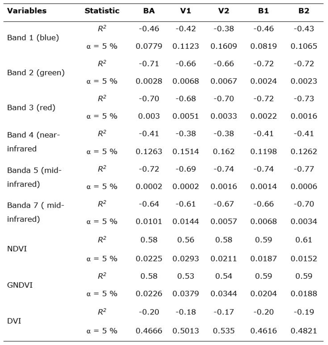
BA = Basal area ha-1; Vi = Volume ha-1; Bi = Biomass ha-1
The mid-infrared (MIR) band was selected as independent variable, as it shows the highest correlation with the forest variables, which made it possible to have the best adjustment statistics in the assessed models. The negative correlation of the mid-infrared band is inversely proportional to forest density, which may be ascribed to the reduction of the albedo in high-density areas (Aguirre et al., 2007; Aguirre et al., 2009). Therefore, a significant increase in the MIR values suggests an increased amount of clorophyll and, consequently, an increase in basal area, volume and biomass. The high associated correlations between the forest parameters (BA, V and B) and the MIR band made it possible to obtain more statistically consistent regression models.
Linear regression models
The spatial distribution of the forest parameters (BA, V and B) of tropical forests is very complex; the topography is one of the main factors affecting the heterogeneity, which makes it difficult to develop an accurate model. However, in this study it was possible to obtain the most statistically consistent regression model for the estimation of the forest variables, which was built using the PROC MODEL procedure of the SAS/ETSTM statistical software package (SAS, 2008).
Table 4 shows the values of the fit statistics and the parameter estimators of the best regression models evaluated for the estimation of the forest variables. The intercept of the model was statistically different from zero (β 0 ), and the rate of change in the slope of the mid-infrared variable (β 1 ) contributed to estimate the variables BA, V and B, as the probabilities associated to the parameters are highly significant in the hypothesis test, at a significance level under 5 % (α=0.05).
Table 4 Fit and statistical values of the assessed models.
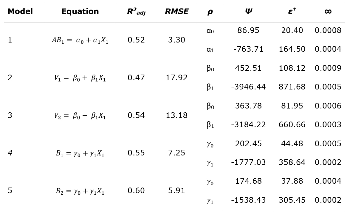
BA 1 = Basal area ha-1; Vi = Volume ha-1; Bi = Biomass ha-1; X1 = Mid-infrared; Ψ = Value of the parameters; ε † = Standard error of the parameters, ∞= Significance level of the parameters.
The five models presented good statistical bases to accurately estimate the forest variables (BA, V and B), which are based on the MIR band, the auxiliary variable (independent variables). However, the prominent models that best describe the biological behavior of the basal area, volume and biomass were models 1, 3 and 5, which obtained the desirable statistics, the highest value for the adjusted determination coefficient (R 2 adj = 0.52, 0.54 y 0.60 for BA, V and B, respectively), and the lowest value for the root of the mean square error (RMSE =3.30, 13.18 and 5.91 for BA, V and B, respectively). These results differ from those obtained by other authors; for example, Muñoz et al. (2014) register higher errors in BA and V, with RMSE = 6.70 m2 ha-1 and 41.45 m3 ha-1 in the temperate forest, based on Spot 4 and 5 images. Aguirre et al. (2007) estimated the BA, V and B using Spot 5 images in Pinus patula Schiede ex Schltdl. & Cham. forests under management, and calculated an RSME of 11.87 m2 ha-1, 96.81 m3 ha-1 and 52.56, Mg ha-1, for BA, V and B, respectively. For their part, Hall et al. (2006) estimated an RMSE of 33.7 Mg ha-1 and 74.7 m3 ha-1 for BA and V, with the support of Landsat ETM imaging. The results obtained by other authors differ from those of the present study, which may be due to the fact that tropical forests, particularly the low deciduous forest, have lower values for BA, V and B than temperate forests.
Figures 2, 3 and 4 correspond to the spatial distribution maps for the basal area (m2 ha-1), volume (m3 ha-1) and biomass (Mg ha-1) of the study area, respectively. The parts in white indicate the non-forest lands (areas without forest cover). Given the range of values for each variable, certain ranges pertain to a one-pixel surface area (900 m2); therefore, their color is imperceptible, and only those areas where the values in which the variable is most abundant are apparent.


Estimation of the forest parameters in terms of total inventories
Table 5 shows the estimations of the total inventory for basal area, volume and biomass obtained using the traditional method (in-field inventory) and the remote sensing method (regression estimators). The mid-infrared (MIR) band had the highest values for correlation with the forest parameters: BA = -0.72, V2 = -0.74 and B = -0.77. Therefore, the regression estimators were built based on the MIR band for the calculation of the BA, V and B. The regression estimator showed the highest precision (permissible error under 10 %) compared to the simple random sampling. Statistically, the two methods produced similar results, although the regression estimator produces more conservative estimations and builds less ample confidence intervals in respect to the total inventory of the SRS (the most optimistic inventory).
Table 5 Comparison between the estimations of the variables (BA m2 ha-1, V m2 ha-1 and B Mg ha-1) based on the traditional and the remote sensing (regression) inventories.
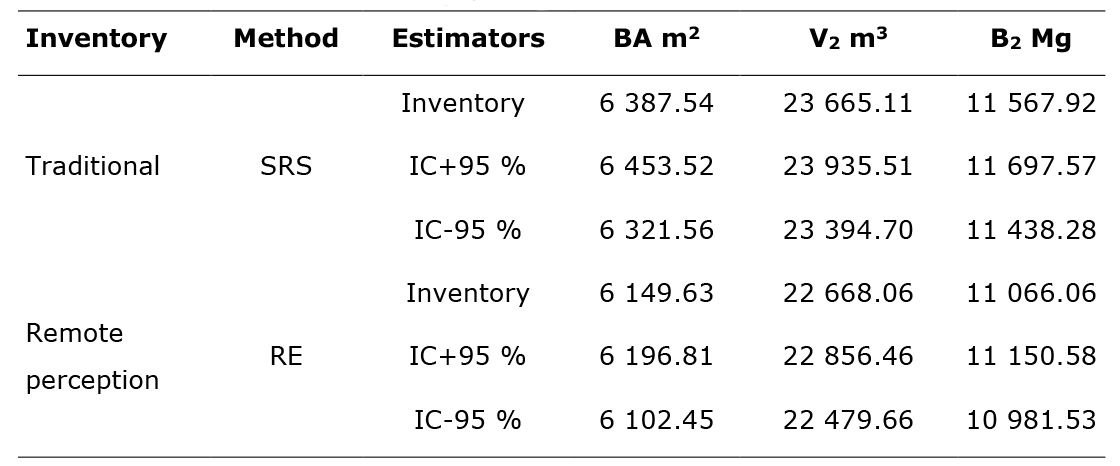
BA1 = Basal area; V1 = Volume; B2 = Biomass; SRS = Simple random sampling; RE = Regression estimator; CI± = Confidence intervals at a level of reliability of 95 %.
The assessment of the forest resources with the support of remote sensing showed more conservative and more accurate results than the traditional inventory (SRS); this allows the forest managers to make better decisions for the sustainable management of the forests and enables them to be integrated in the future into pay-per-service environmental projects through the capture of carbon (Hall et al., 2006: Aguirre et al., 2007).
Conclusions
Five regression models were generated ─one for BA, two for V, and two for B─, and the mid-infrared band of the spectral data and vegetation indexes from Landsat 7 ETM+ images were used as auxiliary variables.
The combinations of data derived from a forest inventory (basal area, volume and biomass) and the satellite image variables (spectral bands and vegetation indices) through linear regression models produce spatial distribution maps for each of the forest parameters.
Acknowledgements
The authors wish to express their gratitude to INIFAP for having authorized the Project “Estimación de biomasa aérea en tres regiones forestales de México” (“Estimation of the aboveground biomass in three forest regions of Mexico”) and granted the corresponding Fiscal Funds in 2015 to finance its execution.
REFERENCES
Aguirre S., C. A., J. R. Valdez L., G. Ángeles P., H. M. de los Santos P., R. Haapanen y A. I. Aguirre S. 2007. Mapeo de variables dasométricas en bosques manejados mediante datos espectrales de Spot 5. Sociedad Latinomaricana en Percepción Remota y Sistemas de Información Espacial Capítulo México. In: Reunión Nacional. SELPER en el Manejo de recursos para el Desarrollo Sustentable. 2007, 22-23 de noviembre. Monterrey, N L .., México. pp. 1-6. [ Links ]
Aguirre S., C. A ., J. R. Valdez L., G. Ángeles P., H. M. de los Santos P., R. Haapanen y A. I. Aguirre S. 2009. Mapeo de carbono arbóreo aéreo en bosques manejados de pino Patula en Hidalgo, México. Agrociencia 43: 209-220. [ Links ]
Aquino R., M., A. Velázquez M., J. F. Castellanos B., H. M. de los Santos P. y J. D. Etchevers B. 2015. Partición de la biomasa aérea en tres especies arbóreas tropicales. Agrociencia. 49:299-344. [ Links ]
Ayala L., R. S., H. J. de Jong B. y H. Ramírez M. 2002. Ecuaciones para estimar biomasa en la meseta central de Chiapas. Revista Chapingo Serie Ciencias Forestales y del Ambiente 7:153-157 . [ Links ]
Comisión Nación Forestal (Conafor). 2011. Manual y procedimientos para el muestreo de campo Re-muestreo 2011. Inventario Nacional Forestal y de Suelos. Zapopan, Jal., México. 140 p. [ Links ]
Comisión Nación Forestal (Conafor). 2012. Inventario Nacional Forestal y de Suelos Informe 2004-2009. Semarnat. Zapopan, Jal., México. 212 p. [ Links ]
Del Ángel-Mobarak, G. A. 2012. La Comisión Nacional Forestal en la historia y el futuro de la política forestal de México. http://www.conafor.gob.mx/biblioteca/documentos/Conafor_ en_la_historia_y_futuro_de_Mexico pdf (10 de abril 2016). [ Links ]
Dong, J., R. Kaufmann, R. B. Myneni, C. J. Tucker, P. E. Kauppi, J. Liskid, W. Buermann, V. Alexeyev and M. K. Hughes. 2003. Remote sensing estimates of boreal and temperate forest woody biomass: carbon pools, sources, and links. Remote Sensing Environment 84:393-410. [ Links ]
Earth Resource Data Analysis Systems (ERDAS). 2011. ERDAS IMAGINE 2011, Version 11.0.2. Hexagon Geospacial. Madison, AL USA. s/p. [ Links ]
García, E.- Comisión Nacional para el Conocimiento y Uso de la Biodiversidad (Conabio). 1998. Climas (clasificación de Köppen, modificado por García). Escala 1:1000000. México. http://www.conabio.gob.mx/informacion/metadata/gis/clima1mgw.xml?_xsl=/db/metadata/xsl/fgdc_html.xsl&_indent=no (16 de mayo 2016). [ Links ]
Gobierno del Estado de México (GEM). 2007. Diagnóstico ambiental del Estado de México por regiones hidrográficas 2007. Tlalnepantla de Baz, Estado de México. 209 p. http://sma.edomex.gob.mx/sites/sma.edomex.gob.mx/files/files/sma_pdf_da_em_2007.pdf (13 de enero de 2017). [ Links ]
Hall, R. J., R. S. Skakun, E. J. Arsenault and B. S. Case. 2006. Modeling forest stand structure attributes using Landsat ETM+ data: Application to mapping of aboveground biomass and stand volume. Forest Ecology and Management 225: 378-390. [ Links ]
Hou, Z., Q. Xu and T. Tokota . 2011. Use of ALS, airborne CIR and ALOS AVNIR-2 data for estimating tropical forest attributes in Lao PDR. ISPRS Journal of Photogrammetry and Remote Sensing 66(6): 776-786. [ Links ]
Instituto Nacional de Estadística y Geografía (Inegi). 2013. Conjunto de datos vectoriales de uso del suelo y vegetación. Escala 1:250 000, Serie V (Capa Unión). Formato vectorial. Aguascalientes, Ags., México. s/p [ Links ]
Instituto Nacional de investigaciones Forestales y Agropecuarias (INIFAP)- Comisión Nacional para el Conocimiento y Uso de la Biodiversidad (Conabio). 1995. Edafología. Escalas 1:250000 y 1:1000000. México. Formato vectorial. México, D.F., México. s/p. [ Links ]
Labrecque, S., R. A. Fournier, J. E. Luther and D. Piercey. 2006. A comparison of four methods to map biomass from Landsat-TM and inventory data in western Newfoundland. Forest Ecology and Management 226: 129-144. [ Links ]
Latifi, H., F. E. Fassnacht, F. Hartig, C. Berger, J. Hernández, P. Corvalán and B. Koch. 2015. Stratified aboveground forest biomass estimation by remote sensing data. International Journal of Applied Earth Observation and Geoinformation 38: 229-241. [ Links ]
Masek, J. G., E. F. Vermote, N. E. Saleous, R.Wolfe, F. G. Hall, K. F. Huemmrich, F. Gao, J. Kutler, and T. K. Lim. 2006. A Landsat Surface Reflectance Dataset for North America, 1990-2000. IEEE Geoscience and Remote Sensing Letters 3 (1): 68-72. doi:10.1109/LGRS.2005.857030. [ Links ]
Muñoz R., M. Á., J. R. Valdez L., H. M. de los Santos P., G. Ángeles P. y A. I. Monterroso R. 2014. Inventario y mapeo del bosque templado de Hidalgo, México mediante datos del satélite SPOT y de campo. Agrociencia 48: 847-862. [ Links ]
Návar C., J. J. 2009. Allometric equations and expansion factors for tropical dry forest trees of Eastern Sinaloa, México. Tropical and Subtropical Agroecosystems 10:45-52. [ Links ]
Ortiz R., A. D., J. R. Valdez L., H. M. de los Santos P., G. Ángeles P., F. Paz P. y T. Martínez T. 2015. Inventario y cartografía de variables del bosque con datos derivados de LiDAR: comparación de métodos. Madera y Bosques 21: 111-128. [ Links ]
Poulain, M., M. Peña, A. Schmidt, H. Schmidt and A. Schulte. 2010. Relationships between forest variables and remote sensing data in a Nothofagus pumilio forest. Geocarto International 25: 25-43. [ Links ]
Protectora de Bosques (Probosque). 2010. Inventario Forestal del Estado de México 2010. Gobierno del Estado de México. Metepec, Estado. de México, México. 93 p. [ Links ]
Statistical Analysis System (SAS). 2008. SAS/STAT® 9.2 User's Guide. SAS Institute Inc. Raleigh, NC USA. n/p. [ Links ]
Razo Z., R., A. J. Gordillo M., R. Rodríguez L., C. C. Maycotte M. y O. A. Acevedo S. 2013. Estimación de biomasa y carbono almacenado en árboles de oyamel afectados por el fuego en el Parque Nacional “El Chico”, Hidalgo, México. Madera Bosques 19: 73-86. [ Links ]
Sinha, S., C. Jeganathan, L. K. Sharma and M. S. Nathawat. 2015. A review of radar remote sensing for biomass estimation. International Journal of Environmental Science and Technology 12(5): 1779-1792. [ Links ]
Sistema Nacional de Trámites (Sinat) 2007. Manifestación de impacto ambiental modalidad regional de los programas de manejo forestal nivel avanzado de ocho ejidos del Estado de Morelos. Semarnat, Zapopan, Jal., México. http://sinat.semarnat.gob.mx/dgiraDocs/documentos/mor/estudios/2007/17MO2007F0002.pdf (15 de abril de 2016). [ Links ]
Šmelko, Š. and J. Merganič. 2008. Some methodological aspects of the National Forest Inventory and Monitoring in Slovakia. Journal of Forest Science 54: 476-483. [ Links ]
Timothy, D., M. Onisimo, S. Cletah and T. S. A. Bangira. 2016. Remote sensing of aboveground forest biomass: a review. Tropical Ecology 57(2): 125-132. [ Links ]
Torres R., J. M. y A. Guevara S. 2002. El potencial de México para la producción de servicios ambientales: captura de carbono y desempeño hidráulico. Gaceta Ecológica 63: 40-59. [ Links ]
Torres R., G., M. E. Romero S., E. Velasco B. y A. González H. 2016. Estimación de parámetros forestales en bosques de coníferas con técnicas de percepción remota. Revista Mexicana de Ciencias Forestales 7(36): 7-24. [ Links ]
United States Geological Survey (USGS). 2015. Landsat data access. http://landsat.usgs.gov/landsat-data-access (20 de mayo de 2015). [ Links ]
Valdez L., J. R., M. J. González G., H. y M. de los Santos P. 2006. Estimación de cobertura arbórea mediante imágenes satelitales multiespectrales de alta resolución. Agrociencia 40:383-394. [ Links ]
Wijaya, A., S. Kusnadi, R. Gloaguen and H. Heilmeier. 2010. Improved strategy for estimating stem volume and forest biomass using moderate resolution remote sensing data and GIS. Journal of Forest Research 21: 1-12. [ Links ]
Received: February 05, 2017; Accepted: April 16, 2017
 Este es un artículo publicado en acceso abierto bajo una licencia Creative Commons
