


Serviços Personalizados
Journal
Artigo
 texto em
  Artigo em XML
 Referências do artigo
 Enviar este artigo por email
Indicadores
-
 Citado por SciELO
 -
 Acessos
Links relacionados
-
 Similares em
SciELO
Similares em
SciELO
Compartilhar

 Permalink
Revista mexicana de ciencias forestales
versão impressa ISSN 2007-1132
Rev. mex. de cienc. forestales vol.10 no.51 México 2019
https://doi.org/10.29298/rmcf.v10i51.223
Articles
A stand density diagram for Pinus patula Schiede ex Schltdl. & Cham.in Puebla, Mexico
1Campo Experimental San Martinito. CIR - Golfo Centro. INIFAP. México.
2Campo Experimental Valle del Guadiana. CIR - Norte Centro. INIFAP. México.
3 Colegio de Postgraduados. Campus Montecillo. México.
4Consultor y Asesor Forestal Independiente. México.
5 Universidad de la Sierra Juárez. Ingeniería Forestal. México.
A stand density diagram (DMD) is a technical tool for applying quantitative silviculture that contributes to improve the technical management of forests; however, the objective was to generate a density management diagram based on Reineke's stand density index to prescribe thinning for Pinus patula stands in Puebla, Mexico. Data from 252 inventory plots in maximum density that covered all growth conditions and the entire age range were processed. Density and quadratic diameter were processed by statistical regression adjusting Reineke’s model. Self-thinning boundaries were fitted and compared to the data with ordinary least squares and stochastic frontier function (SFF) techniques, by Semi-Normal Model (SNM), the Normal Truncated Model (NTM) and the Normal-Exponential Model (NEM) approaches. An evaluation of the quality of statistical and graphical adjustment showed that the stochastic frontier regression technique (SFR) in its semi-normal modality was superior, so it was selected to determine the line of self-thinning. Maximum stand density indexes were 1 078 trees per hectare for a quadratic reference mean diameter of 20 cm. The DMD was generated by defining the different growth zones of Langsaeter. The DMD is useful to manage and prescribe the intensity of thinning as an intermediate silvicultural treatment in terms of the number of trees per hectare to be removed and their equivalent in basal area per hectare for even-aged stands.
Key words: Self-thinning; stand density index; patula pine; stochastic frontier regression; Reineke; even-aged stand
Un diagrama para el manejo de la densidad (DMD) es una herramienta técnica para aplicar silvicultura cuantitativa, la que contribuye a mejorar el manejo técnico de los bosques. El objetivo fue generar un diagrama para manejar la densidad con base en el índice de densidad de rodal de Reineke en bosques coetáneos de Pinus patula en Puebla, México. Se procesó una muestra compuesta por 252 sitios de muestreo para inventario seleccionados en condiciones de máxima densidad, que cubrió todas las condiciones de crecimiento y del intervalo de edades. La información de densidad y diámetro cuadrático se procesó mediante regresión estadística ajustando la relación funcional tamaño-densidad de Reineke. Se comparó la técnica de mínimos cuadrados ordinarios contra la de regresión frontera estocástica en sus modalidades de modelo semi-normal, normal truncado y normal exponencial. Una evaluación de la calidad de ajuste estadístico y gráfico evidenció que la técnica de regresión frontera estocástica en su modalidad semi-normal fue superior, por lo que se seleccionó para determinar la línea de autoaclareo. El índice de densidad máximo fue de 1 078 árboles ha-1 para un Dq de referencia de 20 cm. El DMD se generó con la definición de las diferentes zonas de crecimiento de Langsaeter. El DMD es útil para gestionar y prescribir la intensidad de aclareos como tratamientos silvícolas intermedios, en términos del número de árboles en una hectárea por remover y su equivalente en área basal por hectárea para rodales coetáneos.
Palabras clave: Auto-aclareo; índice de densidad del rodal; pino pátula; regresión frontera estocástica; Reineke; rodal coetáneo
Introduction
Pinus patula Schiede ex Schltdl. & Cham. (patula pine, Mexican weeping pine) is one of the main temperate climate timber conifer species and it is endemic of Mexico. It forms pure even-aged stands or is the dominant species in mixed forests. Its trees have a normal diameter of 50 to 90 cm and a height of 30 to 35 m. Given the abundance, productivity and quality of the forests of this species, its timber is widely utilized for sawing; therefore, it has been used to establish commercial forest plantations (Perry, 1991; Velázquez et al., 2004). Due to its economic importance, a variety of growth and allometric models must be developed and updated as tools for the application of quantitative silviculture, in order to contribute to the planning and improvement of its technical management for purposes of timber production and exploitation.
One of the main tools for forest planning and management that support the decision making process are the diagrams or guides for stand density management and for the prescription of thinnings as intermediate silvicultural treatments (Hernández et al., 2013; Corral-Rivas et al., 2015), especially when applying a regular forest management system. Density is the most important factor that forest managers can manipulate in order to influence the establishment and development of forest species of interest; to improve the quality of the timber and the diameter growth rate, and to influence the timber output by redistributing the growth potential between the remnant individuals (Daniel et al., 1979; Pretzsch, 2009).
Based on the relationship between the density or number of trees (N) per surface area unit and the average size of the trees, it is possible to study the dynamics, the development, the degree of competition and the potential productivity of a stand (Jayaraman and Zeide, 2007; Weiskittel et al., 2009). It is of particular interest to foresters to know the degree of occupation of a site in order to determine the starting time of self-thinning as a result of mortality due to extreme competition in the face of a scarcity of resources such as space, water, nutrients, and sunlight. Under these conditions, an increase in the average size is associated with a progressive reduction of the stand density, up to a given limit (Comeau et al., 2010). In this relationship, the average size can be expressed in terms of the quadratic mean diameter (Dq), estimated with the following equation:
Where:
BA = Basal area (m2 ha-1)
N = Number of trees ha-1
Thus, the ratio is defined by the function:
Where:
α and β = Parameters to be estimated using statistical regression and corresponding to the intercept and to the slope of the line of self-thinning (of maximum intensity or imminent mortality), respectively.
Predefinition of a value for the quadratic diameter of reference (Dr) results in the general expression of Reineke’s Stand Density Index (SDI) as a measure of the relative density and site occupation, defined as the number of trees per hectare for a given mean quadratic mean diameter of reference, to which Reineke (1933) originally assigned a value of 25.4 cm.
This index expresses the ratio of the tree size to the stand density, with the function:
Where:
β, when unknown, can assume the constant theoretical value of 1.605 for any species (Reineke, 1933). However, according to certain authors, the value of the slope may differ significantly between species, and therefore must be estimated for each species and region (Pretzsch and Biber, 2005; VanderSchaaf and Burkhart, 2007; Comeau et al., 2010; Navarro et al., 2011). The index represents both the limit condition of survival and the trajectory of the self-thinning of individual stands; it has the advantage of being independent from the quality of the site and the age of the stand (Long, 1985).
The relative density is defined as the ratio of the current mass density to the maximum density given by the maximum density line for a medium tree size; in the case of the SDI, it is expressed in relation to a predetermined Dq.
In practical terms, the index is a quantitative silvicultural tool of use to forest managers; it allows these to diagnose the status of individual stands in order to manage stand density through the prescription of thinnings as to time and intensity, according to the predefined product to be obtained. The operative tool generated from the SDI is a stand density management diagram (DMD) or guide that provides a method for easily and rapidly comparing, assessing and deciding between different alternative thinning regimes to be implemented in stand density management.
The value of the slope parameter (() has been shown to vary, mainly in terms of the species; therefore, various techniques have been developed for adjusting Reineke’s model in order to improve the definition of the self-thinning line (Santiago-García et al., 2013; Lopes et al., 2016). Another important technical aspect to be considered for adjusting the model is the origin and the selection of the dasometric information to be utilized. Within this context, the purpose of the present study was to generate a density management diagram based on Reineke’s stand density index in natural Pinus patula even-aged stands in Puebla, Mexico, based on the assessment of the quality of adjustment of the size-density model using the ordinary linear least squares and stochastic frontier regression techniques. The DMD will be a technical tool for applying quantitative silviculture that will allow prescribing thinning regimes as intermediate silvicultural treatments, when using a regular management system for this species.
Materials and Methods
Study area
The dasometric information utilized was collected from forest plots with a timber exploitation management program of Forest Management Unit (Umafor) No. 2108, in the region of Chignahuapan-Zacatlán, located in the north of the state of Puebla; geographically, it is located between the parallels 20°07’06” and 19°44’18” N, and the meridians 97°57’18” y 97°38’42” W, in the Hydrological Region RH27 of the basin of the river Tecolutla. This Umafor is constituted by the Asociación Regional de Silvicultores de Chignahuapan-Zacatlán, A.C., (Regional Foresters’ Association of Chignahuapan-Zacatlán) formed by foresters owners of forest plots.
As a result of the current public policy of the federal Mexican government of increasing the timber production and productivity, it has been identified as an important forest supply basin, with the introduction of better practices and intensive silvicultural techniques that may contribute to strengthen and improve forest management.
Sample size and database
A sample consisting of 252 pairs of observations regarding the number of trees and the quadratic mean diameter was processed; it was selected based on a large set of sampling sites for timber inventory, located in forest plots of Aquixtla, Chignahuapan, Ixtacamaxtitlán, Tetela de Ocampo and Zacatlán municipalities; the sites were round, with a surface area of 1 000 m2. Those plots where P. patula formed monospecific, even-aged stands and which, preferably, showed a high density ―a necessary condition to meet the extreme competition requirement due to limited resources― were selected. Furthermore, care was taken to cover all the growth conditions and the entire age interval of the studied species within the observations of the dasometic variables.
In each sampling site, the normal diameter of each and every one of the trees was measured with a 283D/5m-CSE diameter measuring tape and recorded in centimeters; the number of individuals per site was also counted and recorded. Based on this information, a database was generated, and the dasometric variables density or number of trees (N) and quadratic mean diameter (Dq) of the stand were derived per hectare; Table 1 shows their basic statistics.
Table 1 Basic statistics of the dasometric variables analyzed to generate the density diagram of Pinus patula Schiede ex Schltdl. & Cham. stands.
| Variable | Minimum | Maximum | Mean | S.D.1 | V.C2 | Variance |
|---|---|---|---|---|---|---|
| N | 17.00 | 7 466.67 | 689.44 | 1 232.08 | 178.71 | 1 518 013.72 |
| Dq | 4.48 | 71.00 | 30.28 | 13.38 | 44.20 | 179.08 |
1Standard deviation, 2Variation coefficient.
The database was audited, by means of graphic inspection, in order to ensure that the variables of interest exhibited a logical graphic behavior in the shape of an inverted “J” (Figure 1). Thus, it was prepared for the statistical adjustment by regression of the size-density function based on Reineke’s Stand Density Index.

Statistical regression analysis
Reineke’s size-density function expressed in a linear form was adjusted by statistical regression using the ordinary linear least squares (OLS) method; the linearized mathematical structure of Reineke’s model has the form:
Where:
Ln = Natural logarithm function
ε = Error term distributed as ( = idd N(0, σ2)
When the function was adjusted using the stochastic frontier regression (SFR) econometric technique, the following structure of the model resulted:
In this case, the error component is divided into: 1) an error component assumed to account for the technical inefficiency of the data (ui), and 2) an error component associated with the measurement of the individual observations (vi).
vi is assumed as a symmetric disturbance distributed independently of ui; it includes the random variations in production due to factors such as random errors, errors in the observation and measurement of the data; it is assumed to be distributed according to the following equation:
ui is an assymetric term that expresses the technical inefficiency of the observations, and it is assumed to be distributed independently of vi and of the regressors.
Under these assumptions, statistical distributions for ui, distributed to one side only, as in the case of the semi-normal and exponential SFR modality.
If the value of the technical inefficiency ui is assumed to be zero, which is less likely with growing ui values, then the idd N+(0, σ2 u) model refers to the semi-normal model. If the ui (i=1…, N) are not negative random variables idd N+(0, σ2 u), then the model is known as the normal-truncated at zero) (Kumbhakar and Lovell, 2000; Bi, 2004; Pretzsch and Biber, 2005; Zhang et al., 2005).
When the SFR approach was utilized in the statistical adjustment, the Semi-Normal Model (SNM), the Normal Truncated Model (NTM), and the Normal-Exponential Model (NEM) were tested.
Reineke’s size-density function was adjusted by OLS, with the Model procedure of the SAS/ETS® statistical package (Statistical Analysis System, 2011) version 9.3. When SFR was utilized, the function was adjusted using the QLIM procedure of the same statistical package and version. In this case, the algorithm uses the maximum likelihood technique to estimate the frontier and the parameter of technical inefficiency of the observations (ui). In comparison, the SFR technique has the advantage of estimating extreme values (frontier) of a set of data, instead of the mean of a function calculated by the OLS method.
The result and the quality of the adjustment by OLS were compared with the adjustments obtained using SFR; the goodness-of-fit statistics were the value of the logarithm of likelihood (logLik), the Akaike Information Criterion (AIC), and the Schwartz Criterion (SchC), to which, according to Sakici et al. (2008), a rating system was applied, and a total score was obtained for each adjustment modality.
The significance of the parameter and the variances of the error components was also considered, particularly the ratio of the variances of the error components (λ), in addition to the total variance (σ) (Weiskittel et al., 2009; Comeau et al., 2010; Zhang et al., 2013; Quiñonez-Barraza et al., 2018). Furthermore, a graphic comparison of the self-thinning lines generated by each of the adjustment techniques and modalities was carried out in order to reinforce the selection criterion; primarily, the behavior of the trajectory of the self-thinning lines superimposed to the observed data. In the case of the adjustment by OLS, the self-thinning line was determined according to Santiago-García et al (2013), who manually modified the value of the intercept (parameter α), while the value of the slope (parameter β) remained fixed until it a maxα considered to be graphically appropriate was attained.
Based on the values of the parameters of the best adjustment selected on a graph at a logarithmic scale, the line of self-thinning that a hectare can bear without self-thinning, equivalent to a 100 % SDI, was delimited. Subsequently, based on the line of maximum SDI, the lines that defined Langsaeter’s growth areas forming strips of relative densities (four Langsaeter, 1941; Daniel et al., 1979; Smith et al., 1997; Gilmore et al., 2005), where the growth and output of the stands destined to meet the timber production goal will be managed, were estimated. In this manner, the DMD was constructed.
Underutilization area 1 was delimited up to 25 % in relation to the maximum SDI; transition area 2 was defined between 25 and 35 %; area 3, corresponding to the maximum growth of the stand per hectare, was located between 35 and 65 %; area 4, of self-thinning or imminent mortality, was determined at 65 to 100 %. A Dq of reference of 20 cm was used for the construction of the DMD and the definition of the SDI.
Results and Discussion
Adjustment quality and determination of the self-thinning line
The result of the statistical adjustment of Reineke’s size-density function when using the ordinary least squares (OLS) and stochastic frontier regression (SFR) techniques, in the Semi-Normal Model (SNM), Normal Truncated Model (NTM) and Normal-Exponential Model (NEM) modalities, shows that the parameters of the function are significant in all cases (Table 2).
Table 2 Estimated values of the parameters and adjustment statistics for Reineke’s size-density function based on the adjustment by OLS and by SFR.
| Technical adjustment | Parameter | Estimation | Standard error | T value | Significance |
|---|---|---|---|---|---|
| OLS | α | 12.745700 | 0.302450 | 42.14 | <0.0001 |
| β | -2.189370 | 0.090730 | -24.13 | <0.0001 | |
| σ | 0.57644 | ||||
| SFR-SNM | α | 13.502400 | 0.299869 | 45.03 | <0.0001 |
| β | -2.176169 | 0.088676 | -24.54 | <0.0001 | |
| σv | 0.445702 | 0.059947 | 7.43 | <0.0001 | |
| σu | 1.006725 | 0.102813 | 9.79 | <0.0001 | |
| logLik | -280.018350 | ||||
| AIC | 568.036710 | ||||
| SchC | 582.154420 | ||||
| σ | 1.100980 | ||||
| λ | 2.258740 | ||||
| SFR-NTM | α | 13.377648 | 0.312935 | 42.75 | <0.0001 |
| β | -2.179757 | 0.086509 | -25.2 | <0.0001 | |
| σv | 0.486052 | 0.066158 | 7.35 | <0.0001 | |
| σu | 1.437639 | 0.851967 | 1.69 | 0.0915 | |
| μ | -1.945217 | 4.316169 | -0.45 | 0.6522 | |
| logLik | -279.626350 | ||||
| AIC | 569.252690 | ||||
| SchC | 586.899840 | ||||
| σ | 1.517580 | ||||
| λ | 2.957790 | ||||
| SRF-NEM | α | 13.291698 | 0.285911 | 46.49 | <0.0001 |
| β | -2.183796 | 0.084598 | -25.81 | <0.0001 | |
| σv | 0.518719 | 0.050966 | 10.18 | <0.0001 | |
| σu | 0.564340 | 0.078648 | 7.18 | <0.0001 | |
| logLik | -280.051220 | ||||
| AIC | 568.102440 | ||||
| SchC | 582.220150 | ||||
| σ | 0.766520 | ||||
| λ | 1.087950 |
logLik = Logarithm of likelihood; AIC = Akaike Information Criterion; SchC = Schwarz Criterion; σ = Variance of the error estimated as (σ2 u + σ2 v)0.5; λ = Lambda adjustment statistic estimated as the ratio of the variances σu/σv.
However, manual intervention following the adjustment is required in order to define the self-thinning line with the OLS technique because the adjusted line corresponds to the average of the cloud of observed data, and not to the absolute upper limit. This situation causes the determination of this line at the upper frontier of the data to be inefficient, because the value of the intercept is modified using a methodology that considers different criteria, e.g. that the number of trees determined using the maximum SDI should agree (Comeau et al., 2010), or else, increase the value of the intercept in 1.96 standard deviations of the model’s error (Gezan et al., 2007).
These approaches are practical, but they are subjective for estimating the line of self-thinning (Santiago-García et al., 2013; Quiñonez-Barraza et al., 2018). Furthermore, in comparison, the OLS technique is sensitive to the set of observations selected at the density maximum, as, when adjusting the model, a line of self-thinning with an inadequate slope may result (Zhang et al., 2005). For these reasons, the decision was made to select the best adjustment quality between the various tested modalities of the SFR technique, which ensures the direct, immediate obtainment of a maximum absolute line and is technically the correct limit (Bi, 2004; Comeau et al., 2010).
Comparative assessment and a rating system implemented for selecting the best adjustment quality between the different modalities when using SFR revealed that the SNM modality was superior, as it exhibited the lowest values in the adjustment statistics corresponding to the Akaike information criterion (AIC) and to the Schwartz criterion (SchC), as well as to the second best values of the logarithm of likelihood (logLik) of the total variance of the error (σ) and of the variance ratio of the components of the error (λ), along with the high significance of the parameters (tables 2 and 3). Furthermore, it exhibited the lowest variance of the component of the measurement error (σv), and the second lowest value for the variance of the component of the error relative to the technical inefficiency term of the observed data (σu).
Table 3 Comparative evaluation and scores of the goodness-of-fit statistics for the different modalities of the SFR technique analyzed.
| Modality of ajustment |
Score of the adjustment statistics | Total score | ||||
|---|---|---|---|---|---|---|
| logLik | AIC | SchC | σ | λ | ||
| SFR-SNM | 2 | 1 | 1 | 2 | 2 | 8 |
| SFR-NTM | 1 | 3 | 2 | 3 | 3 | 12 |
| SFR-NEM | 3 | 2 | 3 | 1 | 1 | 10 |
logLik = Logarithm of likelihood; AIC = Akaike Information Criterion; SchC = Schwarz Criterion; σ = Variance of the error estimated as (σ2 u + σ2 v)0.5; λ = Lambda adjustment statistic estimated as the ratio of variances (u/(v.
This result was ratified by means of a graphic comparison and visual inspection of the line of self-thinning generated by each adjustment (Figure 2). This confirmed that the adjustment by SFR-SNM exhibited a better pattern, as the line adjusts better to the upper limit of the observed data, having been generated by producing the best definition of the maximum frontier and, therefore, of the line of self-thinning.
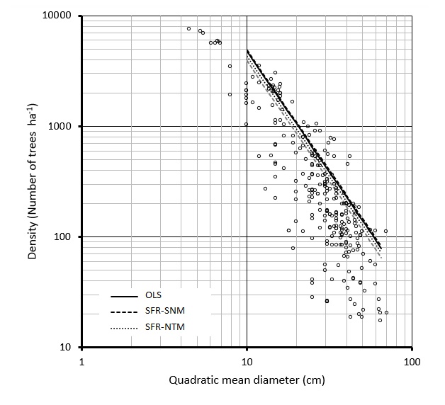
Figure 2 Graphic behavior of the line of self-thinning line generated based on Reineke’s size-density function, using the assessed adjustment techniques.
In this regard, Zhang et al. (2005) point out that this modality of adjustment is the most appropriate regression method for estimating the coefficients of Reineke’s function and subsequently the line of self-thinning, since all the N-q information available on the plots or sites located near the upper limit can be used. According to Burkhart and Tomé (2012), this will eliminate the need to build, in a subjective way, the database for estimating the extreme values of the size-density function. It has been utilized for this purpose on various conifer and broadleaf species (Weiskittel et al., 2009; Comeau et al., 2010; Reyes-Hernandez et al., 2013; Zhang et al., 2013; Lopes et al., 2016; Martínez, 2017).
Wald’s test and the likelihood ratio test proved that the value of the slope (β) of the size-density model estimated by means of SFR-SNM, is statistically different (with α=0.05) from the theoretical value proposed by Reineke (1933), of -1.605. This result agrees with the one recorded by Reyes-Hernandez et al. (2013), who used the same technique and adjustment modality in Picea glauca (Moench) Voss of the Alberta region in Canada, whose slope value was -1.96. However, it differs from the value determined by Santiago-García et al. (2013) for P. patula in the region of Zacualtipán, where the 95 % confidence interval for the slope value of -1.565 ±0.208 included the theoretical value. In this sense, the 95 % confidence interval determined here for this parameter was -1.998 to -2.341, also different from that of -1.714 to -1.910, registered by Quiñonez-Barraza et al. (2018), who used the same technique and modality for a group of species of the genus Pinus in Durango, Mexico.
Within this context, the argument that the slope (β) is not always close to the theoretical value and that it can differ significantly between taxa is reaffirmed (Comeau et al., 2010; Santiago-García et al., 2013), partly due to the fact that different populations have different mortality rates, according to their density, growth habits, site productivity factors, and even the age of the mass (Bi et al., 2000; Weiskittel et al., 2009; Reyes-Hernandez et al., 2013). This leads to the need to develop a particular allometry for each species of interest and, thus, avoid errors when estimating and controlling density (Pretzsch and Biber, 2005).
The maximum SDI estimated with the SFR-SNM adjustment when using a Dq of reference of 20 cm, was 1 078 trees, which differs from that of 1 662 documented by Santiago-García et al. (2013) for the same species in the region of Zacualtipán, Hidalgo, where they determined that the best adjustment technique was SFR in its NTM modality.
The maximum SDI is lower than that estimated for the same species in Huayacocotla, Veracruz, in Monroy’s study (1997) of 1 215 trees with a Dq of reference of 20 cm, in which the function was adjusted in its non-linear form by OLS, with information of 42 temporary sampling sites. Furthermore, the maximum SDI differs from that of the value of 1 603 recorded by Quiñonez-Barraza et al. (2018) for the same site, using the SFR technique in the NTM modality as the best for defining the line of self-thinning.
Construction and use of the stand density management diagram
Based on the line of maximum density, which in this case corresponded to that derived from the adjustment with the SFR-SNM approach, the diagram for the management of the density of monospecific, even-aged P. patula stands was constructed. The number of trees estimated for the limit values as a percentage of the SDI which defines each line delimiting the growth areas, was 270, 380, 700 and 1 078 trees ha-1, for 25 %, 35 %, 65 % and 100 %, respectively; these, in turn, correspond to the lines of free growth (1), transition (2), maximum growth per hectare (3) and self-thinning (4) (Figure 3).
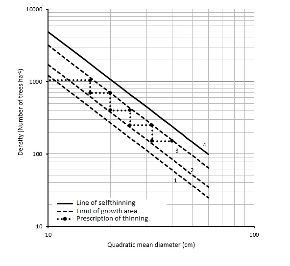
Figure 3 DMD based on Reineke’s SDI for Pinus patula Schiede ex Schltdl. & Cham. and example of the prescription of a thinning program.
This is based on the fact that density management is the most effective means by which the forester can attain the timber production goal of a stand, and on the assumption that the initial density is the basis for prescribing a thinning regime, and that once a thinning has been carried out, there is no mortality due to competition, and therefore the density remains constant until the next thinning.
As an example of the practical and operative usefulness of the DMD, we illustrate how a thinning program is generated as a silvicultural treatment (intermediate fellings). The baseline density (N) is 1 050 trees ha-1, and a theoretical value of Dq=1 cm is assumed; it is equally assumed that, for each stand density, there is a potential maximum average Dq size, or its equivalent in the basal area; therefore, before reaching area 4, of imminent mortality, the first thinning is applied, trying to maintain the residual density at the lower limit of growth area 3 and, in this case, to attain a Dq=16 cm.
From this point on, the mass is allowed to grow until its growth in Dq is once more close to the line of self-thinning and a second thinning is required (Figure 3).
Subsequent thinnings can be carried out based on the same criteria until the maximum growth possible is attained for Dq and the optimal density is achieved. In order to maximize the production, the mass density must be maintained during most of the shift between area 3 and the beginning of area 4.
For the proposed example, Table 3 shows the respective density values and their equivalent in basal area to be removed, as well as the residual value in each thinning, in addition to the corresponding felling intensity. In this case, 150 trees would remain after the final harvest, with an average Dq of 40 cm, equivalent to a basal area of 18.8 m2 ha-1.
Table 3 Thinning program for Pinus patula Schiede ex Schltdl. & Cham., in terms of the number of trees, square diameter and basal area
| Silvicultural treatment |
Density § |
Dq† | I¶ | Trees | Basal area | |||
|---|---|---|---|---|---|---|---|---|
| (N ha-1) | (cm) | (%) | 1 | 2 | 3 | 4 | 5 | |
| Pre-thinning | 1050 - 700 | 1 - 16 | 33 | 350 | 700 | 21.1 | 7.0 | 14.1 |
| First thinning | 700 - 400 | 16 - 20 | 43 | 300 | 400 | 22.0 | 9.4 | 12.6 |
| Second thinning | 400 - 250 | 20 - 25 | 38 | 150 | 250 | 19.6 | 7.4 | 12.3 |
| Third thinning | 250 - 150 | 25 - 32 | 40 | 100 | 150 | 20.1 | 8.0 | 12.1 |
§ = Number of trees before and after the thinning; † = Growth of the quadratic diameter when applying the thinning; ¶ = Thinning intensity; 1 = Number of trees extracted (N ha-1); 2 = Number of remnant trees (N ha-1); 3 = Total basal area (m2 ha-1); 4 = Extracted basal area (m2 ha-1); 5 = Residual basal area (m2 ha-1).
Likewise, the DMD makes it possible to prescribe a thinning program for a stand at a particular development stage; for this purpose, the density per hectare and its respective Dq are determined based on a growth and timber yield system, or using sample sites for timber inventory, estimating the SDI of the target stand; or else, the (N, Dq) point is marked on the DMD according to the growth area where it is located, to determine whether or not thinning is required. Thus, based on the above criteria, different alternative density management regimes are analyzed, and finally the most adequate one is determined according to the management and production goals.
Although the output of the first thinning is not commercial, we must bear in mind that the cost of carrying it out is actually an investment whose return and profits will be reflected in the final harvest. The final thinning must be selective and it must be performed more carefully and with greater technical knowledge. Also, the lower the quality of the site, the longer it will take for a stand to attain the line of self-thinning.
For a given stand, the increase in the stem volume is expected to attain near-maximum values when the relative density is within area (3) (Comeau et al., 2010), a condition in which the trees use the growth space more effectively without exhibiting mortality due to competition. In order to maximize the growth and the increase in volume, the density must be managed by applying thinnings; according to Pérez and Kanninen (2005), this leads to a lower volume estimated per surface area unit, but also to trees with larger diameters and a better shape at younger ages, whereby their value increases.
The frequency and intensity of the thinnings is a compromise between the silvicultural and the financial parts. This will ensure the obtainment of trees with the required size and quality, according to their industrial use, in the shortest time possible. In the practical application of the DMD, the criterion of the technician who manages the stand density is crucial for identifying the trees to be removed, based on the established commercial goals.
Conclusions
In the adjustment of Reineke’s size-density function, the stochastic frontier regression technique in the Semi-Normal Model modality is statistically superior to the ordinary least squares method; therefore, it is a viable alternative for efficiently estimating the upper limit of the line of self-thinning. The stand density management diagram generated based on Reineke’s Stand Density Index for P. patula in the Chignahuapan-Zacatlán region of Puebla, Mexico, will allow an adequate management of the stand density. The diagram is an analytic tool for a quantitative silviculture of immediate practical and operative application; it provides the forester with support for making technical management decisions in P. patula stands because it makes it possible to diagnose and determine the need to carry out thinnings, as well as to establish the intensity of these in terms of the number of trees to be removed and their equivalent in basal area.
Referencias
Bi, H. 2004. Stochastic frontier analysis of a classic self-thinning experiment. Austral Ecology 29(4): 408-417. [ Links ]
Bi, H., G. Wan and N. D. Turvey. 2000. Estimating the self-thinning boundary line as a density-dependent stochastic biomass frontier. Ecology 81(6): 1477-1483. [ Links ]
Burkhart, H. E. and M. Tomé. 2012. Modeling forest trees and stands. Springer. New York, NY USA. 457 p. [ Links ]
Comeau, P. G., M. White, G. Kerr and S. E. Hale . 2010. Maximum density-size relationships for Sitka spruce and coastal Douglas-fir in Britain and Canada. Forestry 83(1): 461-468. [ Links ]
Corral-Rivas, S., J. G. Álvarez-González, J. J. Corral-Rivas, C. Wehenkel y C. A. López-Sánchez . 2015. Diagramas para el manejo de la densidad en bosques mixtos e irregulares de Durango, México. Bosque 36(3): 409-421. [ Links ]
Daniel, T. W., J. A. Helms and F. S. Baker . 1979. Principles of silviculture. 2nd Edition. McGraw-Hill. New York, NY USA. 500 p. [ Links ]
Gezan, S. A., A. Ortega y E. Andenmatten . 2007. Diagramas de manejo de densidad para renovales de roble, raulí y coigüe en Chile. Bosque 28(2): 97-105. [ Links ]
Gilmore, D. W., T. C. O’Brien and H. M Hoganson . 2005. Thinning red pine plantations and the Langsaeter hypothesis: a northern Minnesota case study. Northern Journal of Applied Forestry 22(1): 19-26. [ Links ]
Hernández R., J., J. J. García M. , H. J. Muñoz F., X. García C., T. Sáenz R. , C. Flores L. y A. Hernández R . 2013. Guía de densidad para manejo de bosques naturales de Pinus teocote Schlecht. et Cham. en Hidalgo. Revista Mexicana de Ciencias Forestales 4(19): 62-76. [ Links ]
Jayaraman, K. and B. Zeide . 2007. Optimizing stand density in teak plantations. Journal of Sustainable Forestry 24(4): 1-22. [ Links ]
Kumbhakar, S. C. and C. A. K. Lovell . 2000. Stochastic frontier analysis. Cambridge University Press. New York, NY USA. 333 p. [ Links ]
Langsaeter, A. 1941. Om tynning i enaldret gran-og furuskog. Meddelelser fra Det norske Skogforsøksvesen 8: 131-216. [ Links ]
Long, J. N. 1985. A practical approach to density management. Forestry Chronicle 61(1): 23-26. [ Links ]
Lopes P., E., N. Calegario, G. Saraiva N., E. de Almeida M. and J. de Almeida A . 2016. Estimate of stand density index for Eucalyptus urophylla using different fit methods. Revista Árvore 40(5): 921-929. [ Links ]
Martínez L., J. 2017. Guías de densidad para masas mezcladas de San Pedro El Alto, Zimatlán, Oaxaca. Tesis de Maestría. Postgrado en Ciencias Forestales. Colegio de Postgraduados. Texcoco, Edo. de Méx., México. 99 p. [ Links ]
Monroy R., C. R. 1997. Evaluación de crecimiento y productividad de Pinus patula Schl. et Cham., en la región de Huayacocotla, Veracruz, México. Tesis de Maestría. Facultad de Ciencias Forestales. Universidad Autónoma de Nuevo León. Linares, N.L., México. 120 p. [ Links ]
Navarro C., C., M. A. Herrera, F. Drake A. y P. J. Donoso . 2011. Diagrama de manejo de densidad y su aplicación a raleo en bosques de segundo crecimiento de Drimys winteri en el sur de Chile. Bosque 32(2): 175-186. [ Links ]
Perry, J. P. 1991. The pines of Mexico and central America. Ed. Timber Press. Portland, OR USA. 231 p. [ Links ]
Pérez, D. and M. Kanninen . 2005. Stand growth scenarios for Tectona grandis plantations in Costa Rica. Forest Ecologyand Management 210: 425-441. [ Links ]
Pretzsch, H. and P. Biber . 2005. A re-evaluation of Reineke’s rule and stand density index. Forest Science 51(4): 304-320. [ Links ]
Pretzsch, H. 2009. Forest dynamics, growth and yield: from measurement to model. Springer-Verlag Berlin. Heidelberg, Germany. 664 p. [ Links ]
Quiñonez-Barraza, G. , J. C. Tamarit-Urias, M. Martínez-Salvador, X. García-Cuevas, H. M. de los Santos-Posadas and W. Santiago-García . 2018. Maximum density and density management diagram for mixed-species forests in Durango, Mexico. Revista Chapingo Serie Ciencias Forestales y del Ambiente 24(1): 73-90. [ Links ]
Reineke, L. H. 1933. Perfecting a stand-density index for even-aged forests. Journal of Agricultural Research 46: 627-638. [ Links ]
Reyes-Hernandez, V., P. G. Comeau and M. Bokalo . 2013. Static and dynamic maximum size-density relationships for mixed trembling aspen and white spruce stands in western Canada. Forest Ecology and Management 289: 300-311. [ Links ]
Santiago-García W., H. M. De los Santos-Posadas, G. Ángeles-Pérez, J. R. Valdez-Lazalde, D. H. Del Valle-Paniagua y J. J. Corral-Rivas . 2013. Auto-aclareo y guías de densidad para Pinus patula mediante el enfoque de regresión de frontera estocástica. Agrociencia 47: 75-89. [ Links ]
Sakici, O. E., N. Misira, H. Yavuza and M. Misira . 2008. Stem taper functions for Abies nordmanniana subsp. bornmulleriana in Turkey. Scandinavian Journal of Forest Research 23(6): 522-533. [ Links ]
Statistical Analysis System (SAS). 2011. SAS/STAT® 9.3 User’s Guide. SAS Institute Inc. Cary, NC USA. n/p. [ Links ]
Smith, D. M., B. C. Larson, M. J. Kelty and P. M. S. Ashton . 1997. The practice of silviculture: Applied forest ecology. Ninth Edition. John Wiley & Sons, Inc. New York, NY USA. 537 p. [ Links ]
VanderSchaaf,C. L. and H. E. Burkhart . 2007. Comparison of methods to estimate Reineke's maximum size-density relationship. Forest Science 53(3): 435-442. [ Links ]
Velázquez, A., G. Ángeles, T. Llanderal, A. Román y V. Reyes . 2004. Monografía de Pinus patula. Conafor/Semarnat/Colpos. Jalisco, México. 124 p. [ Links ]
Weiskittel, A., P. Gould and H. Temesgen . 2009. Sources of variation in the self-thinning boundary line for three species with varying levels of shade tolerance. Forest Science 55(1): 84-93. [ Links ]
Zhang, L., H. Bi, J. H. Gove and L. S. Heath . 2005. A comparison of alternative methods for estimating the self-thinning boundary line. Canadian Journal of Forest Research 35(6): 1507-1514. [ Links ]
Zhang, J., W. W. Oliver and R. F. Powers . 2013. Reevaluating the self-thinning boundary line for ponderosa pine (Pinus ponderosa) forests. Canadian Journal of Forest Research 43(10): 963-971. [ Links ]
Received: May 03, 2018; Accepted: November 06, 2018
 Este es un artículo publicado en acceso abierto bajo una licencia Creative Commons
