


Serviços Personalizados
Journal
Artigo
 texto em
  Inglês (pdf)
 Artigo em XML
 Referências do artigo
 Enviar este artigo por email
Indicadores
-
 Citado por SciELO
 -
 Acessos
Links relacionados
-
 Similares em
SciELO
Similares em
SciELO
Compartilhar

 Permalink
Tecnología y ciencias del agua
versão On-line ISSN 2007-2422
Tecnol. cienc. agua vol.9 no.4 Jiutepec Jul./Ago. 2018 Epub 24-Nov-2020
https://doi.org/10.24850/j-tyca-2018-04-03
Articles
Hydrological and hydraulic modeling of an intra-urban river in a transboundary basin using a regional frequency analysis
1Universidad Autónoma de Baja California, Mexicali, Baja California, México, csalazar86@uabc.edu.mx
2Universidad Autónoma de Baja California, Mexicali, Baja California, México, mhallack@mtu.edu
3Universidad Autónoma de Baja California, Mexicali, Baja California, México, alejandro.mungaray@uabc.edu.mx
4Universidad Autónoma de Baja California, Mexicali, Baja California, México, lomeli.marcelo@uabc.edu.mx
5Universidad Autónoma de Baja California, Mexicali, Baja California, México, alopezl@uabc.edu.mx
6Universidad Autónoma de Baja California, Mexicali, Baja California, México, salcedo.adrian@uabc.edu.mx
Floods are among the most recurrent and devastating natural hazards, affecting human lives and causing severe economic damage worldwide. Arid and semi-arid regions are particularly vulnerable to intense storm events over short time periods resulting in flashfloods. These regions represent approximately 30% of the world's area and are inhabited by approximately 20% of the total population. The main objective of this study was to estimate the design storm for return periods of 20, 50, 100, and 500 years, in the semi-arid region of the New River sub-basin, in order to determine the flood areas in the main channel. In this study, an integrated model approach was proposed, consisting of developing a hydrological model for different return periods and performing a regional frequency analysis (RFA) using the L-Moments approach, in order to generate the input for hydrological and hydraulic modeling using the programs HEC-HMS and HEC-RAS. The flood areas obtained ranged from 190.55 ha to 237.83 ha, and depths from 0.10 to 6 meters, which pose a risk to the urban infrastructure of the city. The outcome of this research provides information that can be used by urban planners to reduce flood risks.
Keywords Flood areas; design storm; regional frequency analysis; L-moments; HEC-HMS; HEC-RAS; SIG; simulation
Las inundaciones se encuentran entre los peligros naturales más recurrentes y devastadores, al afectar vidas humanas y causar graves daños económicos en todo el mundo. Las regiones áridas y semiáridas son particularmente vulnerables a tormentas intensas en periodos cortos debido a que provocan inundaciones súbitas. Estas regiones representan un 30% del área mundial y están habitadas por 20% de la población. El objetivo principal del presente estudio es estimar la tormenta de diseño para los periodos de retorno de 20, 50, 100 y 500 años en la región semiárida de la subcuenca del Río Nuevo, a fin de determinar las áreas de inundación del cauce principal. Se propone un modelo integrado, que consiste en desarrollar un acoplamiento del modelo hidrológico e hidráulico para diferentes periodos de retorno, alimentados con un Análisis Regional de Frecuencia (ARF), utilizando el enfoque de los L-momentos, empleando los programas HEC-HMS y HEC-RAS. Las áreas de inundación obtenidas de 190.55 a 237.83 ha y profundidades desde 0.10 hasta 6.0 metros comprometen la infraestructura urbana de la ciudad. Los resultados de esta investigación pueden ser utilizados por organismos encargados de la planeación urbana para disminuir riesgos de inundación.
Palabras clave inundación; tormenta de diseño; análisis regional de frecuencia; L-momentos; HEC-HMS; HEC-RAS; sistema de información geográfica; simulación
Introduction
It is estimated that around 300 million people have been affected since the 1990s due to different natural disasters, and the cost of damages have increased annually until reaching 0.17% of the gross domestic product (GDP) worldwide (Trivedi, Singh, & Indian, 2015).
In accordance with the Intergovernmental Panel on Climate Change (IPCC), deviations from the average weather patterns have been observed worldwide, with a higher frequency of extreme precipitation events in most of the world (UN-HABITAT, 2011). In this sense, floods are among the most devastating and recurrent natural disasters, affecting human lives and causing serious economic damages around the world (Ouma & Tateishi, 2014).
Floods correspond to 50% of the disasters in the world related to water, putting it above famine, droughts, and epidemics, as reported by the United Nations Educational Scientific and Cultural Organization (UNESCO) (Hernández-Uribe, Barrios-Piña, & Ramírez, 2017).
Accelerated population growth and changes in land use patterns have increased human vulnerability to floods, including: mortality and direct morbidity; indirect displacement; and overall damage to crops, infrastructure, and property (Dewan, 2015).
There is a direct relationship between urbanization and changes in hydrological characteristics, such as decreased infiltration, increased runoff, and the increased frequency and height of floods, which in addition to population growth and the accumulation of assets of value, aggravate the risk of flooding in urban areas (Ouma & Tateishi, 2014). In that sense, urban basins are the most vulnerable to these phenomena, mainly due to the dynamics of anthropogenic processes, the disappearance of buffer zones that modify the hydrological response, and the hydraulic behavior of the rivers that run through the city.
Floods can damage and disrupt the transmission and distribution of energy, paralyze transport systems, contaminate drinking water supplies and wastewater treatment facilities, increase the transport of garbage, rubble, and pollutants, and accelerate the spread of water-related diseases (UN-HABITAT, 2011).
In accordance with several authors, arid and semi-arid regions are vulnerable to climatic changes. The precipitation in these regions is primarily characterized by intense storms that typically intensify rapidly, causing flash floods (Pourreza, Samadi, Akhoond, & Ghahraman, 2016). The importance of the arid and semi-arid areas lies in the fact that 20% of the total world population lives there and they represent approximately 30% of the planet’s area (Sivakumar, Das, & Brunini, 2005).
This study was carried out in the Salton Sea transboundary basin located in the semi-arid region of the Colorado River delta, adjacent to the border between the states of Baja California, Mexico and the state of California in the United States. It is estimated that between 10 and 15% of the Salton Sea inlet flow originates in Mexico, and flows north through the New River (The Salton Sea Authority, 2015). The New River is an intra-urban component located in the city of Mexicali, Baja California, México, in northwestern Mexico, which drains surface runoff from local precipitation events, agricultural wastewater, water from industrial processes, and sewage.
The importance of the study in arid areas and semi-arid areas of extreme precipitation events that are high in intensity and short in duration, lies in the damages that these extreme phenomena can cause to populations, urban and agricultural infrastructure, and the economic activities of areas that are important to socioeconomic growth, as is the case of northwestern Mexico and the southwestern portion of the United States.
In the case of Imperial County in the state of California, United States, four states of emergency were declared from 1958 to 2006 due to floods. The residents presented insurance claims of $762 416.00 (US dollars), and the floods damaged roads, sewers, public services, pipes, artificial canals, irrigation systems, and land used for agriculture (Imperial County, 2007). In 2012, a flood that affected around 30% of the crops in Imperial Valley occurred, with losses of more than $7 million dollars (Imperial County, 2013).
The situation in the city of Mexicali is different. Unlike Imperial County, the area with the highest risk of flood is the urban center, since the New River is an intra-urban river, where educational, sports, recreational, commercial, and government infrastructure have been developed, as well as human settlements.
Considering the aforementioned, and coinciding with Jiang et al. (2009), who mentions that flood risk assessment is an important scientific basis for disaster risk management and decision-making by urban planners, the objective of this work was to determine the flood areas in the main channel of the New River, based on a design storm in the transboundary sub-basin, under standard conditions, and with return periods of 20, 50, 100, and 500 years. This study includes the use of L-Moments, which according to Wallis, Shaefer, Barker y Taylor (2007), has demonstrated its reliability for estimating the magnitude of precipitation, because of a significantly increased reliability of in-situ estimations.
In the case of the hydrological and hydraulic analysis of the basin Mulvany (1850), we chose the use of models that allow us to collect and manage a large amount of information on the variables involved in the rain-runoff process, providing data on the spatial distribution of superficial runoff (Vargas-Castañeda, Ibáñez-Castillo, & Arteaga-Ramírez, 2015). We chose to use a semi-distributed hydrological model called the "Hydrologic Modeling System" (HEC-HMS). This program has been widely used to evaluate effects on hydrographs according to possible scenarios related to climate change, type of land use, design and management of hydraulic works, and the delimitation of flood zones (Rodríguez, González, Medina, Pardo, & Santos, 2007; López et al., 2012; Wolfs, Meert, & Willems, 2015).
For the hydraulic simulation, the River Analysis System software (HEC-RAS) was used, a series of components for the one-dimensional flow analyses of rivers, such as: (1) calculation of the constant water flow surface profile and (2) simulation of variable flow.
Area of study
The New River is located in a transboundary area in northwestern Mexico. It consists of different urban centers with different relative weightings. To the north it borders Imperial County in the state of California, United States, and to the south with the city of Mexicali and its agricultural valley in the state of Baja California (Figure 1).

For its part, the Salton Sea basin has an approximate area of 26 432 km2 (Rodríguez-Burgueño, Shanafield, & Ramírez-Hernández, 2017).
According to data from the National Institute of Statistics and Informatics (INEGI), reported in the Population and Housing Census of 2010, the total population in Mexicali was 936 826 inhabitants, representing 29.7% of the total population of the state of Baja California U.S Department of the Interior Bureau of Reclamation, 2012.
The New River is part of the Colorado River delta. This river currently supplies more than 30 million people in the United States and Mexico (Rodríguez-Burgueño, Shanafield, & Ramírez-Hernández, 2017). The Colorado River supplies water to the states of Arizona, California, Colorado, New Mexico, Nevada, Utah, and Wyoming in the United States, and to the states of Baja California and Sonora in Mexico, supplying water to irrigate almost 22 257 km² of agricultural fields and providing more than 4 200 megawatts of electric generation capacity (U.S Department of the Interior Bureau of Reclamation, 2012).
The area of the sub-basin of the New River that flows into the border with the United States is 2 066.69 km² and it has an average slope of 9.61%. The length of its main channel is 47 270 m and its slope is 3.063% (INEGI, 2017). It is worth mentioning that this study covers a section of the New River having a length of 14.17 km, and is geographically located at UTM-WGS84-Z11N, coordinates 3'608,660.30 m north and 645,613.80 m west.
Materials and Methods
A hydrological model was developed to obtain an estimated design cost for different return periods, using a regional frequency analysis with the L-Moments approach. The results were entered into the hydrological and hydraulic modeling of the New River basin to identify the flood zones in the basin’s main channel. The preparation and interpretation of the model’s data for the processing and visualization of geospatial data was facilitated by the use of a geographic information system (GIS) (Heimhuber, 2013). The ArcMap tool and the HEC-GeoHMS and HEC-GeoRAS extensions were used for the preparation of the model’s input files.
The study used historical precipitation records from 35 meteorological stations and flow records from a hydrometric station located in the New River diversion, on the border with the United States. In the case of Mexico, they were obtained through the Rapid Climatological Information Extractor (ERIC III), the Mexican Institute of Water Technology (IMTA), and the National Water Commission (Conagua). The study also included data from a station located at the Engineering Institute of the Autonomous University of Baja California at coordinates 3'611,466.36 m north latitude and 645,886.57 m west longitude. For the United States, the records used corresponded to the years 1930 to 2016, from the California climate data file (CalClim). The basin modeling diagram is shown in Figure 2.
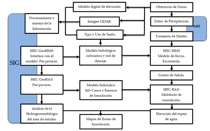
Figure 2 Diagram of hydrological and hydraulic model based on GIS, with design storm obtained through regional frequency analysis (modified from Heimhuber, 2013).
Regional frequency analysis with L-moments approach
Most of the regional frequency analysis procedures try to fit a distribution to the data, whose form is specified from a finite number of indeterminate parameters at the moment of the sample. In particular, asymmetry (skewness) and kurtosis are frequently used to determine the closeness of an observed sample to a postulated distribution. However, statistics are unsatisfactory, because they are algebraically limited by the size of the sample, and in small or moderate samples, it is unusual that the asymmetry and kurtosis of the sample take a value close to the population values (Hosking & Wallis, 1997).
The L-moments, or linear moments, are an alternative system to traditional methods, with conventional moments that characterize the forms of the probability distributions and determine the distribution parameters. According to Hosking and Wallis (1997), L-moments are considered linear combinations of weighted moments. Although L-moments are a relatively recent development in statistics, they form the basis of a mathematical theory and can be used to facilitate the estimation process in regional frequency analyses.
The methodology for the regional frequency analysis used in the present study is based on the work of Wallis et al. (2007), and Schaefer, Barker, Taylor and Wallis (2006), as discussed by Núñez-Cobo Verbist, Ramírez-Hernández, & Hallack-Alegría (2010). It consists of four basic steps: (1) data selection, (2) identification of homogeneous regions, (3) selection of the frequency distribution, and (4) estimation of the quantile function.
Data selection
The analysis begins with the categorization of the sites into
arrangements of possible homogeneous regions using the discrepancy
criteria. Given that the number of stations in the regions can vary, and
the series of data is relatively small, the critical values of
discordance recommended by Hosking and
Wallis (1997) are analyzed, according to the expression
Table 1 Critical discordance values (D i ) according to Hosking and Wallis (1997).
| Number of sites | Critical value | Number of sites | Critical value |
|---|---|---|---|
| 5 | 1.333 | 11 | 2.632 |
| 6 | 1.648 | 12 | 2.757 |
| 7 | 1.917 | 13 | 2.869 |
| 8 | 2.140 | 14 | 2.971 |
| 9 | 2.329 | 15 | 3 |
| 10 | 2.491 |
Identification of homogeneous regions
The criterion of seasonality and the magnitude of the average annual precipitation for the grouping of stations were used. The measures of heterogeneity serve as indicators of the degree of heterogeneity in the L-moments relationships for a group of measurements (Schaefer, Barker, Taylor, & Wallis, 2006). The criterion of homogeneity in this study is based on the work by Wallis et al. (2007), who suggest the ranges presented in Table 2.
Table 2 Critical heterogeneity values (adapted from Núñez-Cobo et al., 2010).
| Heterogeneity | Wallis et al., 2007 |
|---|---|
| Homogeneous | H<2 |
| Possibly heterogeneous | 2<H<3 |
| Heterogeneous | H>3 |
The H1 and H2 statistics measure the relative variability of the
coefficient of L-Cv and L-Skewness (equivalent to the coefficient of
conventional asymmetry) (Núñez-Cobo et
al., 2010) for sites in a sub-region, calculated according to
the expression proposed by Hosking and
Wallis (1997),
These measures compared the observed variability with that expected from a larger sample taken from a homogeneous region represented by the Kappa distribution, according to the 1997 Hosking and Wallis proposal (Schaefer et al., 2006). For this study, one of the criteria used in the integration of homogeneous regions was that the stations that comprise it do not have properties that make them discordant with others that comprise it.
Selection of the frequency distribution
After the identification of the homogeneous regions, the distribution of
the probability for the behavior of the climatic data of interest was
identified. The frequency distribution was chosen based on the diagram
of the L-moment relationship and the goodness-of-fit measure
Table 3 Probability distributions.
| Normal Generalizada |
|
|
| Pearson type III |
|
|
| Generalized extreme value |
|
|
| Four-parameter Kappa |
|
Upper limit |
Estimation of the quantile function
Once the probability distribution for the homogeneous region was
identified, quantiles were determined for different return periods using
the avenues index method, which is expressed as
Hydrological model
The hydrological simulations were carried out using the HEC-HMS 3.2 tool from the Hydrologic Engineering Center. With this took, the rain-runoff process was represented in a simplified way, simulating the hydrogram that occurs at a certain point in the fluvial network as a consequence of an episode of rain (López et al., 2012). This open source software was used since it is considered by many researchers as the most versatile model for modeling the rain-runoff process (USACE, 2016).
The model in HEC-HMS included four components: 1) model of the basin; 2) meteorological model, which indicated the input precipitation required by an element in the sub-basin (Ali et al., 2011); 3) control specification, based on which the starting point and duration of the simulation was determined; and 4) input data, used to provide the hydrological variables observed in the model, such as time series data (USACE, 2016).
Determination of the land use parameters
The modeling of runoff was based on the curve number (CN) method by the Soil Conservation Service (SCS). The CN method is based on the water balance equation, which with the HEC-HMS estimates excess precipitation or effective precipitation as a function of accumulated precipitation, soil cover, land use, and antecedent moisture (Magaña-Hernández, Bá, & Guerra-Cobián, 2013). In order to more precisely determine soil types and estimate the size of their areas and the percentage of each type spatially represented in the area, 1 500 polygons were processed by a GIS, overlaying the land use layer from the National Institute of Geography Statistics and Information Technology (INEGI) and the images obtained through the Google Earth platform. Subsequently, to obtain the CN, the values from the semi-arid regions table (Natural Resources Conservation Service) (NRCS, 1986) were considered. Finally, the model was calibrated by adjusting the CN, since this variable is the most sensitive parameter (López et al., 2012).
For the control specifications of the HEC-HMS, the time lapse and the date of execution of the simulation were defined, with the meteorological model as a representation of precipitation.
The basin model, which is essentially a simplified physical
representation of the basin, was prepared with HEC-GeoHMS. The results
of the model included the runoff hydrology for each sub-basin as well as
graphical and numerical representations of precipitation, loss, and
direct runoff for each sub-basin. The concentration time of the runoff
was calculated with the Kirpich method, where
Delimitation of the sub-basin and micro-basins
A basin is usually delineated with several sub-basins before applying the analysis with the HEC-HMS (Patel, 2009). Therefore, the delimitation of the basins and drainage networks were obtained using an MDE generated from high-resolution elevation data (LiDAR) measuring 5x5 meters, using a GIS (INEGI, 2010).
Hydraulic model
Hydraulic models are used to simulate the behavior of the flow in a river’s main channel and floodplain (Alaghmand, Abdullah, Abustan, & Vosoogh, 2010). The runoff design costs that were generated were used as input for the modeling in HEC-RAS. The geometry of the river was processed using the HEC-GeoRAS extension. Researchers have used this program for the management and use of water resources. The hydraulic model was developed according to three fundamental procedures: Pre-process, process-hydraulic simulation with HEC-RAS, and post-process.
Pre-Process
The geometric data from the hydraulic model were used, which consisted of: the axis of the river, cross-sections, distance of separation between sections, control points, Manning coefficient, and coefficients of contraction/expansion.
Process - Hydraulic simulation with HEC-RAS
In the process stage, the boundary conditions were established upstream and downstream in the modality of permanent flow. It is worth mentioning that, due to the lack of information regarding the water level, the critical water depth was used as the boundary condition (US Army Corps of Engineers) (USACE, 2016). Finally, the mixed flow regime was defined in order to run the modeling. As part of this section, the calibration of the model was carried out by means of the flow-water relationship. The flow was obtained by in-situ measurements using an acoustic Doppler speedometer. The water level was obtained by means of a graduated strip (1 m) installed on the stream. This process was aimed at all parameters or coefficients being adjusted in such a way that the mathematical model reproduced the phenomenon under study (Parhi, Sankhua, & Roy, 2012).
Post - Process
Once the hydraulic model was calibrated, flood maps (depth) were drawn up for the different flow scenarios. The hydraulic modeling in this investigation was carried out without considering the infrastructure of the New River culvert, due to the fact that, in arid and semi-arid regions, flash flood events are caused by high intensity and short duration storms with a high degree of spatial variability. These storms usually present intense floods in very short time frames, even in large basins, resulting in significant amounts of transported sediment, which affects the hydraulic infrastructure of downstream facilities (Maksimovic, 2001). The hydraulic modeling of a 14.17 km segment of the main channel of the New River included a lagoon to the south of the city, which was analyzed by means of 143 cross-sections distributed in approximate intervals of 100 m.
Results and discussion
Flood hazards in arid and semi-arid areas are poorly understood due to the lack of information about their hydrological and hydraulic behavior, affecting the vulnerability of infrastructure projects located in the floodplains (Wang, Zhang, & Baddo, 2016), such as: roads; educational, public services and governmental facilities; private property; and human settlements. The location of the sites exposed to the risk of runoff due to flash floods on the New River’s main channel, and defined by using the hydrological and hydraulic model, are presented below.
Regional Frequency Analysis
The lack of infrastructure at meteorological stations and the limited availability of precipitation records in Mexico complicate the selection of the most appropriate method for analysis. Therefore, a probabilistic approach, such as the regional frequency analysis, is considered as a valid option to estimate the occurrence of an extreme precipitation event, and serves as input for a hydrological model. According to the RFA results, 20 stations were defined in the Salton Sea basin that were considered homogeneous (Table 4), and the Pearson Type III distribution was selected, which was validated with the standard generalized and generalized extreme value functions (The Salton Sea Authority, 2015).
Table 4 Stations in the homogeneous region used in the study.
| Station | North Latitude | West Lenght | PMA | L-CV | L-SKEW | L-KURT | Discordance (Di) |
|---|---|---|---|---|---|---|---|
| Brawley | 634781.34 | 3647110.12 | 47.1 | 0.366 | 0.242 | 0.175 | 0.26 |
| Bataquez | 681308.65 | 3603156.81 | 36.7 | 0.413 | 0.227 | 0.144 | 1.48 |
| Calexico | 643996.85 | 3617742.02 | 44.7 | 0.357 | 0.171 | 0.139 | 0.33 |
| Col Rodríguez | 684677.21 | 3588577.52 | 36.1 | 0.402 | 0.183 | 0.174 | 1.75 |
| Deep Canyon Lab | 557860.08 | 3723635.24 | 84.4 | 0.315 | 0.278 | 0.224 | 1.82 |
| Desert Resort RG | 578003.43 | 3721116.77 | 50.8 | 0.334 | 0.212 | 0.155 | 0.19 |
| Ejido Islitas | 696293.9 | 3581476.88 | 46.0 | 0.361 | 0.234 | 0.236 | 1.14 |
| El Centro 2 | 634674.78 | 3627480.63 | 45.3 | 0.323 | 0.112 | 0.083 | 2.00 |
| Hayfield Pump PL | 627051.03 | 3730180.46 | 65.1 | 0.345 | 0.211 | 0.135 | 0.32 |
| Imperial Airport | 633815.99 | 3635564.07 | 43.1 | 0.317 | 0.144 | 0.122 | 1.00 |
| Indio Fire Station | 538732.66 | 3729969.65 | 50.7 | 0.382 | 0.237 | 0.103 | 1.93 |
| Mecca 2 | 585664.6 | 3714972.54 | 47.8 | 0.386 | 0.175 | 0.148 | 0.90 |
| Mxli (Río Nuevo) | 644499.45 | 3615420.52 | 49.2 | 0.313 | 0.208 | 0.174 | 0.53 |
| Mxli C. Agrícola | 617926.28 | 3602097.2 | 68.7 | 0.354 | 0.239 | 0.214 | 0.48 |
| Niland | 637453.84 | 3683078.33 | 44.5 | 0.358 | 0.265 | 0.222 | 0.79 |
| Ocotillo 2 | 593590.88 | 3623570.42 | 66.5 | 0.333 | 0.186 | 0.194 | 0.66 |
| Ocotillo Wells | 580855.45 | 3668250.7 | 43.5 | 0.310 | 0.147 | 0.123 | 1.11 |
| Palm Springs | 545342.18 | 3743082.29 | 81.2 | 0.343 | 0.253 | 0.125 | 1.85 |
| Presa Morelos | 712686.4 | 3620860.17 | 33.9 | 0.387 | 0.225 | 0.161 | 0.48 |
| Yuma Valley | 713970.32 | 3622219.06 | 49.2 | 0.317 | 0.212 | 0.217 | 0.99 |
Later, the quantiles corresponding to a Tr of 20, 50, 100, and 500 years were defined, which are presented in Table 5.
Table 5 Quantiles corresponding to the return periods of 20, 50, 100, and 500 years
| Quantile | Return periods | Generalized Standard | Generalized extreme value | Pearson Type III | Kappa |
|---|---|---|---|---|---|
| 0.950 | 20.00 | 2.25 | 2.25 | 2.26 | 2.26 |
| 0.980 | 50.00 | 2.79 | 2.81 | 2.75 | 2.79 |
| 0.990 | 100.00 | 3.20 | 3.25 | 3.10 | 3.19 |
| 0.998 | 500.00 | 4.21 | 4.36 | 3.91 | 4.16 |
Characteristics of the hydrological and hydraulic models
Twenty micro-basins were defined with the HEC-GeoHMS extension during the pre-process. The point of interest was located at the outlet of the New River, in the diversion to California, United States, as shown in Figure 3.

Once the physical characteristics of the basin were defined, the project was exported to HEC-HMS, as shown in Figure 4.

Subsequently, the input data for loss, transformation, and routing methods were defined in order to establish the parameters of the model. Then, the different return periods were analyzed, resulting in the maximum costs in the simulations, which served as a basis for the hydraulic analysis (Table 6). It should be noted that in order to increase the accuracy of the CN, the use of a GIS was proposed for the abstraction of the different types of land use, in order to reduce errors due to the generalization of data taken from manuals.
Table 6 Input data for the model: curve number (CN), concentration time (C.T.), initial abstraction (Ia), maximum retention (S), and lag time by micro-basin (inputs), as well as the outputs of the model: drainage area (km2) and maximum costs (m³/s) per return period analyzed.
| Micro-basin | INPUTS | OUTPUTS | ||||||||
|---|---|---|---|---|---|---|---|---|---|---|
| CN | T.C Kirpich (hours) | Lag Time (min) | S | Ia | Drainage Area(km²) | Peak discharge | ||||
| Tr 20 | Tr 50 | Tr 100 | Tr 500 | |||||||
| W650 | 86 | 10.58 | 380.82 | 41.35 | 8.27 | 45.10 | 8.50 | 12.20 | 14.50 | 20.60 |
| W680 | 82 | 12.13 | 436.81 | 55.76 | 11.15 | 29.67 | 4.30 | 6.40 | 7.80 | 11.50 |
| W690 | 82 | 8.28 | 297.91 | 55.76 | 11.15 | 24.09 | 3.50 | 5.20 | 6.30 | 9.40 |
| W730 | 64 | 6.22 | 223.92 | 142.88 | 28.58 | 25.12 | 0.10 | 0.40 | 0.60 | 1.50 |
| W760 | 68 | 10.38 | 373.61 | 119.53 | 23.91 | 37.02 | 1.30 | 2.60 | 3.60 | 6.40 |
| W770 | 88 | 10.54 | 379.48 | 34.64 | 6.93 | 14.49 | 3.10 | 4.40 | 5.10 | 7.20 |
| W780 | 86 | 9.19 | 330.93 | 41.35 | 8.27 | 24.89 | 4.70 | 6.70 | 8.00 | 11.40 |
| W800 | 70 | 11.41 | 410.78 | 108.86 | 21.77 | 26.32 | 0.40 | 0.90 | 1.40 | 2.70 |
| W810 | 86 | 1.36 | 49.01 | 41.35 | 8.27 | 0.29 | 0.10 | 0.10 | 0.10 | 0.10 |
| W840 | 72 | 12.53 | 451.02 | 98.78 | 19.76 | 15.79 | 0.80 | 1.40 | 1.80 | 3.10 |
| W860 | 88 | 10.26 | 369.23 | 34.64 | 6.93 | 16.67 | 3.60 | 5.00 | 5.90 | 8.20 |
| W880 | 72 | 12.31 | 443.21 | 98.78 | 19.76 | 27.47 | 0.70 | 1.40 | 2.00 | 3.60 |
| W900 | 77 | 11.69 | 420.96 | 75.87 | 15.17 | 27.40 | 2.70 | 4.40 | 5.50 | 8.50 |
| W910 | 82 | 11.84 | 426.12 | 55.76 | 11.15 | 37.76 | 5.50 | 8.20 | 9.90 | 14.70 |
| W960 | 68 | 10.80 | 388.98 | 119.53 | 23.91 | 29.76 | 0.30 | 0.80 | 1.30 | 2.60 |
| W1000 | 76 | 9.75 | 350.98 | 80.21 | 16.04 | 20.44 | 0.80 | 1.40 | 1.90 | 3.20 |
| W1010 | 78 | 19.21 | 691.70 | 71.64 | 14.33 | 54.20 | 5.90 | 9.30 | 11.50 | 17.70 |
| W1020 | 82 | 10.24 | 368.81 | 55.76 | 11.15 | 25.94 | 2.60 | 4.00 | 4.90 | 7.60 |
| W1130 | 80 | 8.68 | 312.59 | 63.50 | 12.70 | 22.22 | 1.50 | 2.40 | 3.10 | 5.00 |
| W1180 | 70 | 28.22 | 1015.91 | 108.86 | 21.77 | 60.38 | 1.70 | 3.20 | 4.40 | 7.80 |
| TOTAL | 565.02 | 34.20 | 51.20 | 62.10 | 92.30 | |||||
Determination of flood zones by return period
Even though flood hazards in arid and semi-arid zones are poorly understood due to the lack of information about their hydrological and hydraulic behavior, they affect the vulnerability of the infrastructure located in the flood plains. Therefore, this type of analysis is necessary in order to locate the areas exposed to the risk of runoff associated with flash floods. In the case of the New River main channel, these zones were defined using a coupling of the hydrological and hydraulic models, as presented below.
The depths and the flood areas for the different return periods analyzed are shown in Table 7, which shows that for a return period of 500 years, the depth reached 6.0 meters and the flooded area was 237.83 ha, while for 20 years, the depth reached 4.80 meters and the flooded area was 190.55 ha.
Table 7 Flood areas and depths for each return period analyzed.
| Tr | Flood Area (ha) | Depth range (m) |
|---|---|---|
| 20 | 190.55 | 0.10 - 4.80 |
| 50 | 206.25 | 0.10 - 5.20 |
| 100 | 216.66 | 0.10 - 5.50 |
| 500 | 237.83 | 0.10 - 6.00 |
The next figures show the representation of the flooded areas for return periods of 20 and 500 years, as well as the minimum and maximum depths obtained in the study (Figure 5).
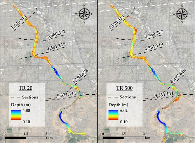
Figure 5 Size of the flood area and depth distribution generated by HEC-RAS for events with return periods of 20 and 500 years.
Figure 6, Figure 7, Figure 8, Figure 9 and Figure 10 show the hydraulic simulation for five large sites by means of the cross-sections 1 520.513, 3 360.577, 4 581.119, 8 292. 628 and 9 334.141, on the New River channel. As can be seen, the stream is defined by steep slopes on the east and west banks of the stream. Also seen are the flood areas that affect the city's infrastructure with a return period of 20 years. The depths of the water are also presented for each return period analyzed and each section, with the modeling in HEC-RAS.
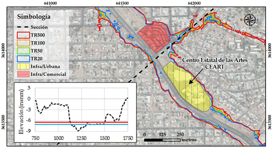
Figure 6 Flooded areas corresponding to 1 520.513 section, affecting commercial and urban infrastructure.
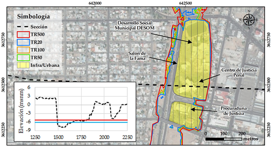
Figure 7 Flooded areas corresponding to a 3 360.577 section, with urban effects (public buildings and sports facilities).
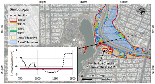
Figure 8 Flooded areas in a 4 581.119 section with effects on human settlements and educational infrastructure (human settlements with approximately 200 families).
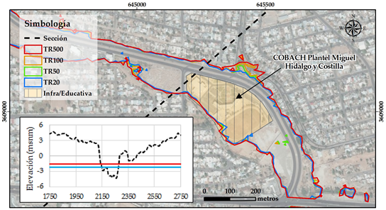
Figure 9 Flooded areas corresponding to section 8 292.628 with effects on educational infrastructure.

Conclusions
With the support of an RFA and L-Moments, the inputs can be obtained for hydrological and hydraulic models in an area with few weather stations and historical information records. Therefore, the RFA is a useful and reliable tool for identifying the different return period quantiles and estimating the height of the precipitation that will be used as input in the hydrological model. It is worth mentioning that the management of the GIS information system using the HEC-GeoRAS and HEC-GeoHMS extensions enabled the preparation of the input data for the coupling of the hydrological model HEC-HMS with the hydraulic model in HEC-RAS. The result of this coupling of models for the semi-arid region in the transboundary basin of the New River is relevant because it is the first time it has been done, and therefore, it is expected to serve as a basis for future hydrological and hydraulic analyses of the area.
The accelerated growth of the city is a determining factor in the increase of impermeable sites in some areas of the urban area, and in the volume of runoff discharge. Therefore, it is recommended to periodically evaluate and adjust the CN of each micro-basin, particularly in the urban areas surrounding the runoff.
Although it is true that the increase in the magnitude of the precipitation for the return periods of 20, 50, 100, and 500 years generated increases in the volume of discharge, the flood area did not increase significantly. This is because the main channel of the New River is defined by pronounced slopes on its eastern and western banks. Therefore, the most significant threat identified in an extreme precipitation event in the New River is related to the depth of the water, which could reach 4.80 m for a TR of 20 years and 6.0 meters for a TR of 500 years. It should be mentioned that the increase in depth during these precipitation events represents a threat to this area, given the development of roads, human settlements, public and private buildings that house government activities, and educational facilities. Another immediate effect relates to the roads that connect the city from east to west, and intersect in the New River, since according to the flood maps, there is a road discontinuity that divides the city in two parts, making communication difficult. This result can be observed in any of the four return periods analyzed.
It is proposed that this analysis be carried out at the micro-basin level to establish the level of water logging and flooding in different parts of the city. In addition, the hydraulic behavior of the New River embankment should be analyzed by including it as one of the input variables of the model, in order to optimize the results obtained in HEC-RAS.
The results of this research will be useful to urban planners and municipal, state, and federal authorities, as well as civil protection systems and society in general, in order to make decisions concerning the management of strategies aimed at preventing disasters and to take steps that provide comprehensive solutions to the management of the risks associated with flash floods.
Referencias
Alaghmand, S., Abdullah, R., Abustan, I., & Vosoogh, B. (2010). GIS-based river flood hazard mapping in urban area (a case of study in Kayu Ara River Basin, Malaysia). International Journal of Engineering and Technology, 2(6), 488-500. [ Links ]
Dewan, T. (2015). Societal impacts and vulnerability to floods Blangladesh and Nepal. Weather and Climate Extremes, 7, 36-42. [ Links ]
Heimhuber, V. (2013). GIS based flood modeling as part of an integrated development strategy for informal settlements (tesis de maestría). Technische Universität München, Múnich, Alemania. [ Links ]
Hernández-Uribe, R., Barrios-Piña, H., & Ramírez, A. (2017). Análisis de riesgo por inundación: metodología y aplicación a la cuenca Atemajac. Tecnología y Ciencias del Agua, 8(3), 5-25. [ Links ]
Hosking, J. R. M, & Wallis, J. R. (1997) Regional frequency analysis: An approach based on l-moments. Cambridge, UK: Cambridge University Press. Recuperado de http://dx.doi.org/10.1017/cbo9780511529443 [ Links ]
Imperial County. (2013). Imperial County Multi-Jurisdiction Hazard Mitigation Plan Update. Recovered from http://www.co.imperial.ca.us/announcements%5CPDFs%5CImperialCountyMHMPUpdate2013_121913.pdf [ Links ]
INEGI, Instituto de Estadística, Geografía e Informática. (2010). Imagen Lidar. México, DF, México: Instituto de Estadística, Geografía e Informática. [ Links ]
INEGI, Instituto de Estadística, Geografía e Informática. (2017). Simulador de Flujos de Agua de Cuencas Hidrográficas. Recuperado de http://antares.inegi.org.mx/analisis/red_hidro/siatl/# [ Links ]
López, J. J., González, M., Scaini, A., Goñi, M., Valdenebro, J., & Gimena, F. N. (2012). Caracterización del modelo HEC-HMS en la cuenca de río Arga en Pamplona y su aplicación a cinco avenidas significativas. Obras y Proyectos, 12, 15-30. [ Links ]
Magaña-Hernández, F., Bá, K., & Guerra-Cobián, V. H. (2013). Estimación del hidrograma de crecientes con modelación determinística y precipitación derivada de radar. Agrociencia, 47, 739-752. [ Links ]
Maksimovic, C. (2001). Urban drainage in arid and semi-arid climates, 40(2). París, Francia: Organización de las Naciones Unidas para la Educación, la Ciencia y la Cultura, UNESCO. [ Links ]
Malekinezhad, H., & Zare-Garizi, A. (2014). Regional frequency analysis of daily rainfall extremes using L-moments approach. Atmósfera, 27(4), 411-427. [ Links ]
Mulvany, T. J. (1850). On the use of self-registering rain and flood gauges. Proceedings of the Institution of Civil Engineers, 4(2), 1-8. [ Links ]
NRCS, Natural Resources Conservation Service. (1986). Technical release 55. Washington, DC, USA: U.S. Department of Agriculture. [ Links ]
Núñez-Cobo, J., Verbist, K., Ramírez-Hernández, J., & Hallack-Alegría, M. (2010). Guía metodológica para la aplicación del análisis regional de frecuencia de sequias basado en L-momentos y resultados de aplicación en América latina. Montevideo, Uruguay: Organización de las Naciones Unidas para la Educación, la Ciencia y la Cultura, UNESCO. [ Links ]
Ouma, Y., & Tateishi, R. (2014). Urban flood vulnerability and risk mapping using integrated multi-parametric AHP and GIS: Methodological overview and case study assessment. Water, 6(6), 2073-4441. [ Links ]
Parhi, P., Sankhua, R., & Roy, G. (2012). Calibration of channel roughness for Mahanadi River (India), using HEC-RAS model. Journal of Water Resource and Protection, 4(10), 847-850. [ Links ]
Patel, K. (2009). Watershed modeling using HEC-RAS, HEC-HMS, and GIS models-A. New Jersey, USA: Rutgers, The State University of New Jersey. [ Links ]
Pourreza, B. M., Samadi, S. Z., Akhoond, A. M., & Ghahraman, A. B. (2016). Reliability of semiarid flash flood modeling. Journal of Hydrologic Engineering, 22(4), 05016039. [ Links ]
Rodríguez, S., González, P., Medina, N., Pardo, C., & Santos, R. (2007). Propuesta Metodológica para la generación de mapas de inundación y clasificación de zonas de amenaza. Caso de estudio en la parte baja del Río Las Ceibas (Neiva-Hulia). Avances en Recursos Hidráulicos, 16, 65-78. [ Links ]
Rodríguez-Burgueño, J. E., Shanafield, M., & Ramírez-Hernández, J. (2017). Comparison of infiltration rates in the dry river bed of the Colorado River Delta during environmental flows. Ecological Engineering, 106, 675-682. [ Links ]
Schaefer, M. R., Barker, B. L., Taylor, G. H., & Wallis, J. R. (2006). Regional precipitation-frequency analysis and spatial mapping of precipitation for 24-hour and 2-hour durations in Eastern Washington. Washington, DC, USA: Washington State Department of Transportation. [ Links ]
Sivakumar, M. G., Das, H., & Brunini, O. (2005). Impacts of present and future climate variability and change on agriculture and forestry in the arid and semi-arid tropics. Climate Change, 31-72. DOI 10.1007/1-4020-4166-7_4 [ Links ]
The Salton Sea Authority. (2015). A brief description of its current conditions, and potential remediation projects. Recovered from http://www.sci.sdsu.edu/salton/SaltonSeaHomePage.html [ Links ]
Trivedi, A., Singh, A., & Indian, A. (2015). Analysis of key factors for waste management in humanitarian response: An interpretive structural modelling approach. International Journal of Disaster Risk Reduction. DOI: 10.1016/j.ijdrr.2015.10.006 [ Links ]
UN-HABITAT, United Nations Human Settlements Programme (2011). UN-Habitat Annual Report 2010. Nairobi, Kenya: United Nations Human Settlements Programme. [ Links ]
US Department of the Interior Bureau of Reclamation. (2012). Colorado River Basin Water Supply and Demand Study. Washington, DC, USA: The U.S. Department of the Interior. [ Links ]
USACE, US Army Corps of Engineers. (2016). HEC-RAS River Analysis System User’s Manual Version 5.0. US Army Corps of Engineers. Hydrologic Engineering Center. Washington, DC, USA: US Army Corps of Engineers. [ Links ]
Vargas-Castañeda, G., Ibáñez-Castillo, L. A., & Arteaga-Ramírez, R. (2015). Development, classification and trends in rainfall-runoff modeling. Ingeniería Agrícola y Biosistemas, 7(1), 5-21. DOI: 10.5154/r.inagbi.2015.03.002 [ Links ]
Wallis, J. R., Schaefer, M. G., Barker, B. L., & Taylor, G. H. (2007). Regional precipitation- frequency analysis and spatial mapping for 24 hours and 2 hours durations for Washington State. Hydrology & Earth System Sciences, 11(1), 415-442. [ Links ]
Wang, M., Zhang, L., & Baddo, T. D. (2016). Hydrological modeling in a semi-arid region using HEC-HMS. Journal of Water Resource and Hydraulic Engineering, 105-115. Recuperado de http://dx.doi.org/10.4314/jfas.v9i2.27 [ Links ]
Wolfs, V., Meert, P., Willems, P. (2015). Modular conceptual modelling approach and software for river hydraulic simulations. Environmental Modelling and Software, 71, 60-77. [ Links ]
Received: October 20, 2017; Accepted: February 14, 2018
 Este es un artículo publicado en acceso abierto bajo una licencia
Creative Commons
Este es un artículo publicado en acceso abierto bajo una licencia
Creative Commons
