Introduction
Geomagnetic storms are perturbations on the Earth’s magnetic field caused by the southward component of the interplanetary magnetic field (IMF). They can last from a few hours to several days (Gonzalez et al., 1999). This magnetic field orientation allows magnetic reconnection (Akasofu, 1981) and energy transfer from the solar wind tbo the Earth’s magnetosphere causing a depression of the Earth’s magnetic field horizontal (H) component due to the diamagnetic effect generated by the azimuthal circulation of particles in the ring current (Gonzalez et al., 1994; Echer et al., 2008). Thus, a geomagnetic storm can be defined by ground-based low-latitude geomagnetic field horizontal component variations (Gonzalez et al., 1994). Based on this definition, the disturbance storm time index (Dst) is established as the average of the disturbance variation of the H-component, divided by the average of the cosines of the dipole latitudes at the observatories for normalization to the dipole equator (Sugiura & Kamei, 1991). Dst index serves as a good measure of the overall strength of near-Earth electric currents, especially the ring current (Sugiura, 1964) and it is obtained from four selected geomagnetic observatories operating in the equatorial region (Sugiura & Kamei, 1991).
Another index that can register the geomagnetic activity occurring during a storm is the auroral electrojet index. This index measures the global electrojet activity in the auroral zone (Davis & Sugiura, 1966) and is also derived from geomagnetic variations in the H-component observed from selected observatories throughout the auroral zone in the northern hemisphere (Pallocchia et al., 2008). The auroral electrojet index is represented by four índices: AU, AL, AE and AO. The AU and AL indices (Davis & Sugiura, 1966), are used to express the strongest current intensity of the eastward and westward auroral electrojets, respectively (Pallocchia et al., 2008). The AE index defined as AE=AU-AL (Davis & Sugiura, 1966) provides an estimate of the overall horizontal current strength, and to some extent, a rough measure of the ionospheric energy losses (Ahn et al., 1983), while the AO index defined as AO=(AU+AL)/2 (Davis & Sugiura, 1966) provides a measure of the equivalent zonal current (Menvielle et al., 2011).
The mentioned indices have long records that allow statistical studies of the causes of geomagnetic activity and their related phenomena. In other studies, the relationship between the Dst and AE indices shows that there is a correlation (with a correlation coefficient of 0.87) for these indices during the recovery phase of the geomagnetic storms (Akasofu, 1981; Saba et al., 1997). Thus, correlations between the geomagnetic indices and possible drivers provide the basis for its prediction. In this way, different computational tools have been used for this purpose during the past decades, such as artificial neural networks (ANN). Several examples of the application of ANN to forecast the Dst index can be reviewed in (Kugblenu et al., 1999; Lundstedt, 2005; Sharifi et al., 2006; and references therein). Revallo et al., (2014) proposed one of the most recent works on this subject. They present a method for forecasting Dst index 1-hour ahead using an ANN combined with an analytical model of the solar wind-magnetosphere interaction.
In this work, Dst index 1 to 6 hours ahead were forecasted by an ANN using the time series of the past values of Dst itself and AE index as input parameters. This ANN was optimized with genetic algorithms (GA) to update the ANN weights. A genetic algorithm is an optimization technique based on the evolutionary ideas of natural selection and genetics (Holland, 1975). The algorithm repeatedly modifies a population of individual solutions into a search space by relying on bio-inspired operators such as mutation, crossover, and selection (Davis, 1991). Due to facts, GA may offer significant benefits over the more typical search of optimization algorithms, and it can be used to optimize the update weights process of an ANN with better results than the traditional back-propagation algorithm (Lazzús, 2016). With this, we propose an improved method to forecast the Dst variation based on measurements at ground level. As far as we know, no application yet exists for forecasting Dst index using a hybrid ANN+GA method, as is presented here.
Neural networks and genetic algorithms
In this study, we utilize of a multilayer feed-forward neural network. This ANN consists of one input layer with N inputs, one hidden layer with q units and one output layer with n outputs. The output of this model can be expressed as (Lazzús, 2016):
where W nj are the weights between unit j and unit n of the input and hidden layers, W ji are the weights between the hidden layer and the output, and B j and B n represent the biases of the hidden and output layer, respectively. The activation functions f n (x) and f j (x) are linear or nonlinear. We used one hidden layer with f j (x) as a tangent hyperbolic nonlinear activation function and f n (x) as a linear function in the output layer. For a given set of D inputs, we define the root mean square error (RMSE) by:
where y real denotes the actually given output and y calc the neural network output. This network was trained to minimize RMSE, replacing the gradient descent error by genetic algorithms (GA), and considering that GA have been applied in the optimization of ANN obtaining better results than the commonly used back-propagation algorithm (Lazzús, 2016). Note that, traditional optimization techniques such as back-propagation learning algorithm (BPLA) can determine the number of network parameters too, such as network connection weights, but BPLA is neither able to control the parameter optimizations in the absence of gradient information nor to reduce the problems of trapping of local minima during the convergence process. In contrast, GA is able to solve these problems.
GA was developed by Holland (1975), and based on the natural selection in biological systems. This algorithm uses genetic information to find new search directions into an error surface aided by operators that reflect the nature of the evolutionary process, such as reproduction, crossover, and mutation (Lazzús, 2016).
GA generates a population of individuals, whose characteristics are encoded in a fixed-length bit string by emulating the biological genotype (Davis, 1991). As a parallel to nature, genetic material is swapped between the individuals and mutated to produce offspring, with corresponding changes in their phenotypic performance (Lazzús, 2016). The crossover operator is an analog of the recombination of genetic material as observed in reproduction. Crossover involves splitting the genomic bit-strings of two parents at a given number of locations and then splicing together complementary sections of each parents’ bit-string to form the genotype of the new individual. Crossover occurs with a random probability, and the mutation operator simulates natural mutation of DNA. This simply involves flipping bits in the string in a stochastic manner. The mutation should be fairly infrequent and should be applied following crossover (Davis, 1991).
The main differences between GA and other optimization algorithms are: i) only the objective function and the corresponding fitness levels influence the directions of search; ii) it uses probabilistic transition rules, not deterministic ones; and iii) it works in an encoding environment of the parameter set rather than the parameter set itself (Lazzús, 2016).
Database and training
Data sets of geomagnetic Dst index and AE index were taken from the World Data Center for Geomagnetism of Kyoto (WDC, 2016), and used to train the network. Figure 1 shows the time series used. These series contain 233,760 hourly data indices from 00 UT on 01 January 1990 to 23 UT on 31 August 2016.
A cross-validation method was used to calculate the predictive capabilities of the proposed method. The training set contains 175,320 hourly data points from 00 UT on 01 January 1990 to 23 UT on 31 December 2009, while the prediction set contains 58,440 hourly data points from 00 UT on 01 January 2010 to 23 UT on 31 August 2016. According to the largest decay values of Dst index, the storms fall into low (Dst>-20nT), medium (-20nT>Dst>-50nT), high (-50nT>Dst>-100nT), and extreme (Dst<-100nT) categories (Jankovičová et al., 2002). Table 1 shows the storm ranges for the database used. Here, geomagnetic indices cover a wide range of values, from -422nT to 95nT for the Dst index and from 3nT to 3195nT for the AE index. Figure 2 shows the hourly data points categorized as geomagnetic events (extreme storms) that contain the training and prediction sets. In this Figure, both sets show a great number of extreme storms with levels of Dst<-100nT.
Table 1 Data ranges and geomagnetic storm levels present in the database used.
| Data ranges | Training set | Prediction set |
|---|---|---|
| No. data points | 233,760 | 58,440 |
| ∆Dst (nT) | -422 to 66 | -374 to 95 |
| ∆AE (nT) | 5 to 3,195 | 3 to 2,227 |
| Geomagnetic storm levels (Jankovičová et al., 2002) | ||
| Dst>-20nT | 117,338 | 47,007 |
| -20nT>Dst>-50nT | 46,329 | 9,774 |
| -50nT>Dst>-100nT | 9,765 | 1,519 |
| Dst<-100nT | 1,888 | 140 |
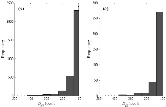
Figure 2 Histograms of main geomagnetic storms. (a) Dst levels for the training set, and (b) Dst levels for the prediction set.
The main problem of the time series study consists on predicting the next value of the series up to a specific time by using the known past values of the series itself (Palit & Popovic, 2005). In our case, the goal of the proposed method is to use the past values of the time series of geomagnetic indices (t‒τ b ,...,t‒1,t), with τ b =0,1,…,K, to predict the geomagnetic index Dst(t+ τ a ), with τ a =1,2,…,T.
The inputs are normalized using the following equation:
where X i is the input data i, and X i min and X i max are the smallest and largest data values, respectively. Next, the inputs (N) are processed for the ANN neurons as in Eq. (1), and subsequently, GA is used to obtain optimum weights W and biases B for the ANN.
The steps to calculate the optimum weights and biases using GA are as follows (Lazzús, 2016):
1) The initial weights in the ANN are randomly generated (initial population). Then, M-chromosomes are also randomly generated to represent this population, with each chromosome representing all the initial weights and biases in the ANN, which are optimized by GA. Let M be the size of population, i.e. M groups of weights and biases are initialized and encoded into chromosomes as Z m (k)={W ij ,W nj ,B j ,B n }, with m=1,…, M, and they are randomly distributed in the solution space.
2) The chromosome fitness is evaluated by the performance of the ANN during the training. In this case, fitness function F is defined as F m (Z m (k))=1/(y real -y(k) calc )2.
3) Fitness function value of each individual in the population is evaluated and the best individual chromosomes are selected for mating. The selection is repeated until the number of individuals in the mating pool is the same as the number of individuals in the population (Che et al., 2011). Here, the probability that parental individuals have been selected is given as p m =F m /∑M =1 F m (Yang et al., 2016).
4) Two individuals Z u (k) and Z v (k) are selected from the mating pool to generate two child individulas Z u (k+1) and Z v (k+1) by two-point crossover, using L as the length of chromosome and a random integer value in interval [1, L] (Yang et al., 2016). We used a two-point crossover operator to prevent unreasonable children, two chromosomes break from two points, and thus new chromosomes are generated from the crossover of the first part of parents (Che et al., 2011). Thus, two crossover points are selected, the binary string from beginning of chromosome to the first crossover point is copied from one parent, the part from the first to the second crossover point is copied from the second parent and the rest is copied from the first parent (Meng et al., 2007).
5) A mutation operator is applied to maintain diversity within the population. Since the initial weights of the ANN could take any values between 0 and 1, the mutation is conducted by switching random genes. The approximate optimal solutions can be found quickly in order to set up the mutation rate as a parameter to control mutation probability (Eiben et al., 1999). Here, the mutation strategy for Z m (k+1) is given as Z m (k) if r>r mu , or Z m (k)×[Z p (k)+Z q (k)] if r≤r mu , where r is a random number in interval [0,1], and r mu is the mutation factor. Also, Z p (k) and Z q (k) are randomly selected from the population and computed as the different gene [Z p (k)+Z q (k)]. Then, Z m (k)×[Z p (k)+Z q (k)] is compared with Z m (k) by item. When r>r mu the item in Z m (k) remains unchanged, otherwise the item in Z m (k) mutates to corresponding item in Z m (k)×[Z p (k)+Z q (k)]. Thus, a new individual Z m (k+1) emerges after comparison (Yang et al., 2016).
6) Finally, root mean square error (RMSE) is calculated for all the individuals’ value. When RMSE is less than the preset value, it is considered that the population has converged to the set including the global optimal solution in the ANN+GA (Lazzús, 2016).
Figure 3 shows a block diagram of the ANN+GA method developed for this study. In GA, the number of individuals, the crossover operator, the crossover probability, the mutation operator, and the mutation probability, summarize the main parameters to synchronize for their application in a given problem (Lazzús, 2016). For this task, an exhaustive trial-and-error procedure was applied for tuning the GA parameters employed in the ANN. Table 2 shows the selected parameters of ANN+GA. Importantly, these values were obtained from a sub set of examples.
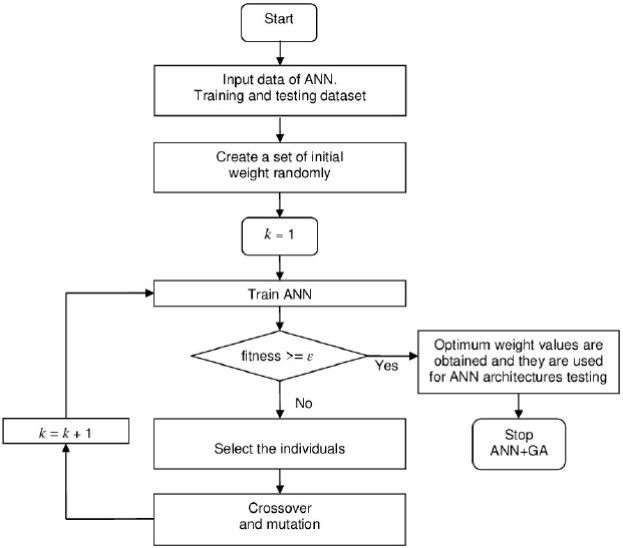
Figure 3 Flow diagram for training of our ANN using GA. Note that training and prediction sets are loaded at the same time by the ANN+GA program, but it must be made clear that only data from the training set were used during the training phase and only prediction data were used in the prediction phase.
Table 2 Parameters used in the hybrid ANN+GA.
| Section | Parameter | Value |
| ANN | NN-type | feed-forward |
| Number of hidden layers | 1 | |
| Maximum learning epoch | 2000 | |
| Transfer function (hidden) | Tansig | |
| Transfer function (output) | Linear | |
| Normalization range | [-1, 1] | |
| Weight range | [-10, 10] | |
| Bias range | [-5, 5] | |
| Minimum error | 1e-4 | |
| GA | Population | 10 |
| Crossover operator | two point | |
| Crossover rate | 0.8 | |
| Mutation operator | binary | |
| Mutation rate | 0.2 | |
| Fitness function | RMSE |
From the above methodology, several network architectures were tested to select the most accurate scheme. The most basic architecture normally used for this type of application involves a neural network consisting of three layers (Lazzús, 2013). The number of hidden neurons needs to be sufficient to ensure that the information contained in the data was adequately represented. No specific approach to determine the number of neurons in the hidden layer (NHL) exists, but many posible alternative combinations do. Here, the optimum NHL was determined by adding neurons systematically (as a cascade approach) and by evaluating the RMSE during the training process (Lazzús, 2016). Thus, we trained 10 different networks for each architecture, from 1 to 30 hidden neurons, totaling 300 NNs (or replications) for each problem (Dst(t+1), Dst(t+2),…, Dst(t+6)). In addition, ANN+GA was trained for 2000 epochs (100 generations) for each problem.
Results and discussion
Once the training process was successfully completed and the optimal architecture was determined, the prediction set containing data not used in the training set was evaluated. Table 3 summarizes the best results obtained during the training and prediction processes for forecasting the Dst index from 1 to 6 hours in advance.
Table 3 Summary of statistical results obtained in the forecast of Dst (t+1 to t+6).
| Ahead | Input | NHL | Training set | Prediction set | ||
| RMStra | Rtra | RMSEpre | Rpre | |||
| t+1 | t-4 | 3 | 4.63 | 0.983 | 3.38 | 0.980 |
| t+2 | t-6 | 9 | 7.71 | 0.952 | 6.12 | 0.946 |
| t+3 | t-6 | 12 | 9.72 | 0.923 | 8.63 | 0.918 |
| t+4 | t-8 | 18 | 10.31 | 0.914 | 10.12 | 0.901 |
| t+5 | t-8 | 24 | 12.54 | 0.889 | 11.67 | 0.879 |
| t+6 | t-9 | 27 | 14.23 | 0.841 | 13.72 | 0.832 |
The results show that the ANN+GA method can forecast the Dst from 1 to 6 hours ahead with a good accuracy by according to the results obtained via RMSE tra and RMSE pre . Note that the period from 01 January 1990 to 31 December 2009 (training set) present a greater occurrence of geomagnetic storms with levels of -50nT> Dst >-100nT (high) and Dst <-100nT (extreme), while for the period used in the prediction set (from 01 January 2010 to 31 August 2016), the occurrence of these types geomagnetic storms are less frequent. Because of this, the prediction RMSE were smaller than the training RMSE.
As in Table 3, and considering the results obtained during the training and prediction steps (RMSE tra and RMSE pre , respectively), deviation increases with the time-ahead. From these results, we observe that our network can forecast only up to 4 hours in advance quite precisely, by considering correlation coefficient R greater than 0.9. Note that similar results were obtained by Stepanova & Pérez (2000). For us these results are only related to the processing capabilities of neural networks, and have no relation with the dynamics of the magnetosphere. To clarify, in order to predict each case (from 1 to 6 hours ahead), we trained a new network.
In particular, we focus our analysis on the forecast of Dst(t+1), since for this case we have obtained the best results and can compare them with other available methods. Thus, for this case the best input vector obtained to solve Dst(t+1) was:
To clarify, for all cases the best input vector was derived from the weights matrices of the network, by using the methodology described above. For Dst(t+1), these input parameters, we obtained the optimum architecture of 10-3-1, with 10 input neurons corresponding to 5 input parameters for Dst index (t‒4, t‒3,...,t‒0) and 5 other input parameters for AE index, 3 others neurons in the hidden layer, and one output neuron for Dst(t+1), as shown in Table 3. Note that considering the structure of this ANN, its length of chromosome was L=10×3+3×1+3+1=37. Also, for this forecast, in Figure 4 appears a comparison between real (solid line) and calculated values (dots) of Dst(t+1) obtained with the proposed ANN+GA method. Fig. 4a shows the comparison during the training step between predicted and real values of Dst(t+1), from 00 UT on 01 January 1990 to 23 UT on 31 December 2009. Here, R was 0.983, while the slope of the curve (m) is 0.967 (expected to be 1.0). Fig. 4b shows the comparison in the prediction step between predicted and real values of Dst(t+1), from 00 UT on 01 January 2010 to 23 UT on 31 August 2016). In this case, R was 0.979 while m was 0.965.
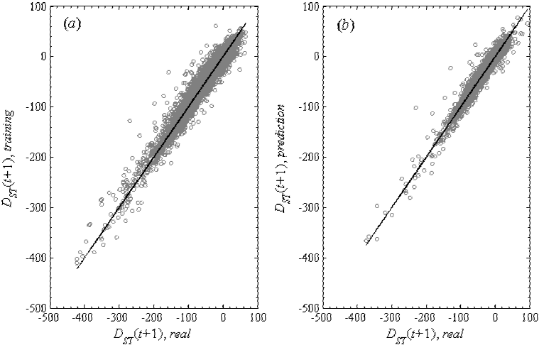
Figure 4 Comparison between real and calculated values of Dst(t+1) using ANN+GA: (a) training set and (b) prediction set.
To distinguish the predictive capabilities of ANN+GA between different storm levels, an exhaustive analysis according to storm type for Dst(t+1), as well as. A comparison between our results and the ones obtained via persistence method was made. Note that the persistence method is usually used in forecast applications. Thus, Table 4 shows the correlation coefficients obtained with the proposed ANN+GA method according to geomagnetic storm levels for Dst(t+1) versus the results obtained using the persistence method for the same datasets. The results show that the ANN+GA method is a very powerful tool for making forecasts of different geomagnetic storm types. Notably, in the forecast of extreme storms (Dst<-100nT), our results were highly accurate with correlation coefficients R of 0.945 for the training process and R of 0.937 for the prediction step.
Table 4 Statistical results obtained with the proposed ANN+GA and the persistence method according to geomagnetic storm levels for Dst(t+1).
| Storm levels (Jankovičová et al., 2002) | Training set | Prediction set | ||
| Rpers | RANN+GA | Rpers | RANN+GA | |
| Dst>-20nT | 0.932 | 0.938 | 0.937 | 0.949 |
| -20nT>Dst>-50nT | 0.840 | 0.878 | 0.838 | 0.870 |
| -50nT>Dst>-100nT | 0.802 | 0.864 | 0.807 | 0.842 |
| Dst<-100nT | 0.905 | 0.945 | 0.863 | 0.937 |
As test case to evaluate the predictive accuracy of our ANN+GA method in the forecast of Dst index, we used the extreme geomagnetic event of March 2015. The St. Patrick’s Day storm on 17 March is categorized as G4-NOAA level that corresponds to an extreme storm (Dst<-100nT). This geomagnetic storm serves ou proposed for two main reasons: i) it was the first strongest geomagnetic storm of solar cycle 24, and ii) space weather agencies around the world failed to predict it (Jacobsen & Andalsvik, 2016). Figure 5 shows the recorded values of the solar wind plasma, the magnetic field, and the geomagnetic indices during the St. Patrick’s Day storm from 16-20 March 2015 (OMNI, 2016). The indices contained in this Figure are typically used for monitoring the behavior of a geomagnetic storm. Importantly, the source of this storm must be traced back to a coronal mass ejection (CME) event that occurred on 15 March 2015 at ~2:10 UT and was caused by a partial halo CME with a propagation speed of ~668 [km/s] (Wu et al., 2016). Later, an interplanetary (IP) shock arrived to Earth (at ~04:45 UT) causing the sudden storm commencement (Nava et al., 2016; Wu et al., 2016), as indicated by the solid vertical line in Fig. 5. Next, Dst values decreased right after the IMF turned southward (Dst=~80nT) and intensified during passage through the region between the IP shock and its driver (Wu et al., 2016), as indicated by the dashed vertical line in Fig. 5. Afterwards, it recovered slightly after the IMF turned northward. A few hours later, the IMF turned southward again due to the strongly negative Bz associated with a magnetic cloud (MC) and caused a second storm intensification, reaching a Dst peak of -223 nT on March 17 (Nava et al., 2016; Wu et al., 2016), as the dotted vertical line in Figure 5 reveals.
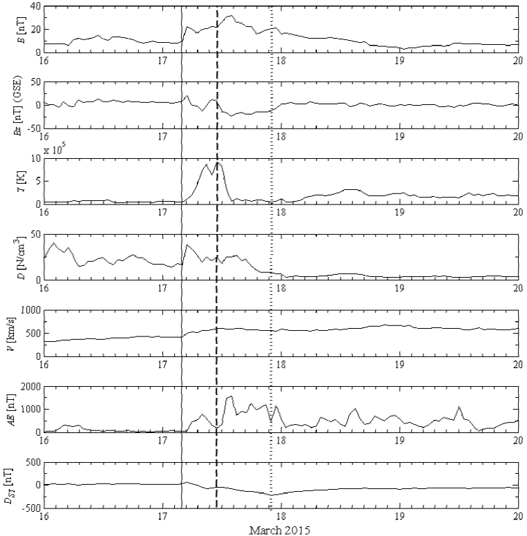
Figure 5 Recorded values of the magnetic field, the solar wind plasma, and the geomagnetic indices during the St. Patrick’s Day geomagnetic storm (OMNI, 2016). From top to bottom panels: magnetic field magnitude (B), Bz of the field in GSE, proton temperature (T), proton density (D), flow speed (V), AE index, and Dst index.
Figure 6 shows the forecast of the Dst index during the St. Patrick’s Day storm by using our proposed method. As observed, this storm evolves from an abrupt variation of the Dst index toward negative values until reaching a minimum value (the main phase of the storm), and starts its recovery until reaching again a Dst value close to zero (the recovery phase of the storm). Note that this complete behavior was correctly and quite accurately forecasted by ANN+GA for both phases, where for all forecasted cases of Dst (t+1 to t+6), our method obtains RMSE≤10nT and R≥0.9 both for the main phase and the recovery phase of that geomagnetic storm (see, Figure 6). It should be made clear that data from this storm did not form part of the training set and were completely unknown to the network. This Figure thus also provides a general view of the accuracy and capabilities of the proposed method to forecast the complete behavior of any geomagnetic storm.
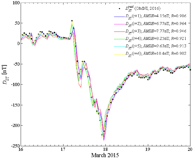
Figure 6 Forecasting of the St. Patrick’s Day geomagnetic storm using the proposed ANN+GA method from 1 to 6 hours in advance.
On the other hand, various models have been developed to forecast Dst index (e.g, in Kugblenu et al., 1999; Lundstedt, 2005; Sharifi et al., 2006; and references therein). However, comparative studies on ANN and the traditional regression approaches for forecasting the Dst index have also been conducted, and it has been shown that ANN methodology offers a promising alternative to the traditional approach (Lundstedt, 2005; Stepanova et al., 2005). In this way, a comparison can be made between the proposed ANN+GA method and related methods available in the literatura. For example, Wu & Lundstedt (1996) obtained a RMSE=16nT in the prediction of Dst(t+1) using 97 selected storms. Similarly, Stepanova & Pérez (2000) obtained R from 0.95 to 0.72 for a selected set of geomagnetic storms taken from 1983. Later on, Stepanova et al. (2005) predicted Dst(t+1) with R from 0.7 to 0.8. Also, Temerin & Li (2006) obtained RMSE=6.65nT and R=0.914 in the forecast of Dst(t+1) during the years 1995-2002. Jankovičová et al. (2002) present a R=0.95 for years 1998-1999. Most recently, Revallo et al. (2014) obtained R of 0.77 in the forecast of Dst(t+1) using storms between 1998 to 2005. Meanwhile, our proposed ANN+GA method shows a general accuracy of >97% with RMSE=3.4nT and R=0.98 in the forecast of Dst(t+1). It must be mentioned that our results were obtained from different methodologies and databases, and all these results cannot be compared directly with one another. However, from the partial statistical analysis of these different methods, we conclude that our proposed method generates reasonably accurate results. In addition, a comparison was made between the ANN+GA method, and a neural network with standard back-propagation (BPNN) with similar architecture and database. Thus, for example, this BPNN shows a RMSE of 5.95, and a R of 0.962 in the forecast of Dst(t+1) with architecture 10-3-1. Figure 7 shows the correlation coeficients obtained by ANN+GA method versus persistence and BPNN methods in the forecast of Dst ((t+1) to (t+6)). This Figure proves that the ANN+GA method can forecast the Dst index more accurately than persistence and BPNN methods. Thus, all these results provide a tremendous increase in the accuracy of the forecast of Dst index, and show that both the ANN application and the appropriate selection of the independent input vector were crucial. The innovative aspect introduced in this study pertains to use of a hybrid neural model plus genetic algorithm with only two input variables (Dst and AE) and a limited number of neurons in the hidden layer for forecasting the Dst index.
Conclusions
Based on the results presented in this study, the following main conclusions obtain: i) The proposed ANN+GA method can be properly trained for forecasting the Dst index quite accurately (RMSE≤10nT and R≥0.9); ii) The geomagnetic indices (Dst and AE) used have influential effects on the good training and predicting capabilities of the selected network; iii) The ANN+GA method can forecast the Dst index more accurately than persistence and BPNN methods; iv) The low deviations found with the proposed method indicate that it can predict the future values of Dst index more accurately than others ANN approach proposed in the literature.


 nueva página del texto (beta)


