SciELO - Scientific Electronic Library Online

 
vol.67 número3Temperature profiles due to continuous hot water injection into homogeneous fluid-saturated porous media through a line sourceNew magnetic flux flows with Heisenberg ferromagnetic spin of optical quasi velocity magnetic flows with flux density índice de autoresíndice de materiabúsqueda de artículos
Home Pagelista alfabética de revistas  

Servicios Personalizados

Revista

Articulo

Indicadores

Links relacionados

  • No hay artículos similaresSimilares en SciELO

Compartir


Revista mexicana de física

versión impresa ISSN 0035-001X

Rev. mex. fis. vol.67 no.3 México may./jun. 2021  Epub 21-Feb-2022

https://doi.org/10.31349/revmexfis.67.369 

Research

Gravitation, Mathematical Physics and Field Theory

Solitary wave solutions in two-core optical fibers with coupling-coefficient dispersion and Kerr nonlinearity

S. Abbagaria  b 

A. Houwec 

H. Rezazadehd 

A. Bekire 

S. Y. Dokaf 

aDepartment of Basic Science, Faculty of Mines and Petroleum Industries, University of Maroua, P.O Box 08, Kaélé, Cameroon,

b Laboratory of Mechanics, Materials and Structures, Department of physics, University of Yaounde I, P.O. Box 812, Yaounde, Cameroon. e-mail: abbagaris@yahoo.fr

cDepartment of Physics, Faculty of Science, the University of Maroua, P.O Box 814, Maroua, Cameroon. e-mail: ahouw220@yahoo.fr

dFaculty of Engineering Technology, Amol University of Special Modern Technologies, Amol, Iran. e-mail: rezazadehadi1363@gmail.com

eNeighbourhood of Akcaglan, Imarli Street, Number: 28/4, 26030, Eskisehir, Turkey. e-mail: bekirahmet@gmail.com

f Department of Physics, Faculty of Science, The University of Ngaoundere, Ngaoundere, Cameroon. e-mail: numami@gmail.com


Abstract

This paper studies solitary wave solutions in two-core optical fibers with coupling-coefficient dispersion and intermodal dispersion. To construct bright, dark and W-shape bright solitons, the couple of nonlinear equations describing the pulses propagation along the two-core fiber have been reduced to one equivalent equation. By adopting the traveling-waves hypothesis, exact analytical solutions of the generalized nonlinear equation (GNSE) were obtained by using three relevant mathematical methods, namely, the auxiliary equation method, the modified auxiliary equation method and the sine-Gordon expansion approach. Lastly, the behavior of the soliton solutions was discussed and some contours of the plot evolution of the bright, W-shape bright and dark solitons are obtained.

Keywords: Two-core optical fiber; soliton solutions; nonlinear Schrödinger equation

PACS: 04.20.Jb; 05.45.Yv; 94.05.Fg

1.Introduction

The single fiber that hold two parallel cores is knowing as two-core optical fiber. Nowadays, a lot off attention have been focussed to the devices based on two-core fibers. Thus, some authors have been demonstrated that the double-core single-mode can be tailored as a directional coupler, polarization splitters and power depend nonlinear couplers 1. Furthermore, investigation of solitary waves in two-core optical fiber have been advanced beyond measure, such as soliton shape and mobility control in optical lattices 2, dark and bright solitons 3,4 and so on. Moreover, these localized solutions in optical fibers usually take the forms of shift solitons, spatiotemporal soliton, temporal soliton and spatial soliton 5. More recently, some works have been done to build soliton in a nonlinear coupler in a presence of a raman effect and solitary waves in asymmetric tin-core fibers 6,7. Today, analytical investigation of solitary waves become a big challenge, that is while some relevant methods have been used to construct exact solutions for partial differential equations (PDEs), such as unified method 8,9, initial condition field distributions 10, the simplest equation approach 11, the split-Step method 12, the first integral method 13, new extended direct algebraic scheme 14,15 and the generalized tanh method 16, just to name a few.

The following pair of nonlinear Schrödinger equations describes the pulse propagation through the two-core optical fibers 17. The model has been studied by Samir et al. 18, and novel traveling-waves solutions have been retrieved by help of Jacobian elliptic functions.

ia1x-β222a1t2+γ|a1|2a1-ca1+ik1a2t=0,\naia2x-β222a2t2+γ|a2|2a2-ca2+ik1a1t=0, (1)

where a1(x,t) and a2(x,t) represent the slowly envelopes of the electric field. However, x and t are, respectively, the propagation distance and time in a retarded frame. The parameter β2 accounts for normal-or anomalous-GVD at the carrier frequency. γ=2πn2/(λAeff) controls the self phase modulation (SPM), where λ, n2 and Aeff are, respectively, free-space optical wavelength, nonlinear refractive index of the fiber material and the effective area of each core, while c stands for the coupling coefficient and it is also proportional to the spatial encroachment between the mode fields in the two-core 18. Here k1=dc/dω accounts for the coupling-coefficient dispersion (CCD) at the carrier frequency and corresponds to the intermodal dispersion which arises from the group-delay difference between the only and uneven super-modes of the two-core fiber 18. Recently, it has been obtained a photonic bandgap two-core fiber when the coupling coefficient is equal to zero 19. More recently, some authors have investigated solitons in dual-core fiber by adopting the traveling wave method, and results for dark and bright solitons have been found 20.

We aim in this paper to construct solitary waves and discussed the behavior of the results obtained along with the constraint relation. To do so, we surmise a1(x,t)=a2(x,t)=a(x,t), hence the set of couple of the generalized nonlinear Schrödinger equation which describing pulses propagating in two-core fibers reduces to one equivalent equation

iax-β222at2+γ|a|2a-ca+ik1at=0. (2)

To obtain the travelign wave solutions of (2), the following ansatz is adopted:

a(x,t)=ϕ(ξ)exp[ifξ],ξ=x-vt, (3)

where v is the velocity frame. Hence the phase f(ξ) can be written in the following form

δω(x,t)=-(f(ξ))t. (4)

By inserting (3) into (2), we obtained the following set of equations

-ϕf'-β22v2ϕ''+β22v2ϕf'2+γϕ3-cϕ+k1vϕf'=0, (5)

and

(1-k1v)ϕ'-β2v2ϕ'f'-β22v2ϕf''=0. (6)

Multiplying (6) by ϕ and integrating once with the constant of integration having a value of zero, it is obtained:

f'=(1-k1v)β2v2, (7)

and thus, (4) gives

δω=(1-k1v)β2v. (8)

The formula given for (7) depends on β2, which measures the GVD at the carrier frequency ( β2<0 stands for anomalous dispersion and β2>0 for normal dispersion), and the coupling coefficient dispersion (CCD) corresponds to the intermodal dispersion occuring from the group-delay difference between the even and odd supermodes of the two-core fiber. However, when the value of CCD is equal to zero, the phase corresponds to the specific operating condition for a conventional two-core fiber design 21. To investigate analytical solutions which could propagate in two-core fiber optic, we substitute (7) into (5), which leads to the following ODE.

-β22v2ϕ''\na-12(2cv2β2+v2k12-2vk1+1)β2v2ϕ+γϕ3=0. (9)

So, the following section adopted three relevant integration techniques, namely, the auxiliary equation method, the modified auxiliary equation method and the sine-Gordon expansion approach to derive bright and dark soliton solutions and we will discuss the behavior of the results obtained.

2.Glimpse of the methods

2.1.The auxiliary equation method

The following steps describe the auxiliary equation method 26,27. Considering a given nonlinear partial differential equation (NPDE) with independent variables (x,t) and dependent variables a(x,t)

P(a,ax,at,axt,axx,att)=0. (10)

Step 1: The traveling-wave solution of (10) is used in the following form

a(x,t)=ϕ(ξ),ξ=x-vt, (11)

where v is the traveling-wave speed. Then (10) was converted into a nonlinear ordinary differential equation as follows

N(ϕ,ϕ',ϕ,ϕ,......)=0. (12)

Step 2: Suppose that the exact solutions of (12) can be expressed

ϕ(ξ)=i=0nAi(g(ξ))i, (13)

and g(ξ) satisfies the following auxiliary equation

gξ=2(C0+C1g+C2g2+C3g3+C4g4), (14)

gξξ=C1+2C2g+3C3g2+4C4g3, (15)

with gξ=(g/ξ), Ci(i = (0,1,2,3,4)), A0, Ai (i = 1,2,…n) are real constants to be determined later.

Step 3: Under the terms of the method, it is assumed that the solution of Eq.(12) can be written in the following form

ϕ(ξ)=A0+A1g(ξ)\na+A2g(ξ)2+A3g(ξ)3+.......Ang(ξ)n, (16)

where A0,A1,A3,A4, and A n are real constants to be determined later. To calculate the value of n, we balance the highest-order nonlinear terms in (12), and then the value of n can be determined.

Step 4: Substituting (16), (15) and (14) into (12) provides a polynomial of g(ξ). Next, collecting all the coefficients g(ξ)i, (i=0,1,2,........n) forms a system of algebraic equations. Solving this system, we describe the variable coefficients of A0, A i , i = (1,2,……,n), so the solution to (12) can be obtained in terms of g(ξ).

Step 5: To obtain the exact solutions to (10), the following solutions of (14) or (15) are used.

Case 1: for C0=C1=C3=0,C2>0,C4<0,

g(ξ)=-C2C4\sech(2C2ξ), (17)

Case 2: for C0=(C22/4C4),C1=C3=0,C2<0,C4>0,

g(ξ)=-C22C4tanh(-C2ξ). (18)

Case 3: for C0=C1=0C2>0,C4>0,

g(ξ)=C2sech2(2C2ξ2)2C2C4tanh(2C2ξ2)-C3. (19)

Case 4: for C0=C1=0,C2>0,C32-4C2C4>0,

g(ξ)=2C2sech(2C2ξ)C32-4C2C4-C3\sech(2C2ξ). (20)

Case 5: for C0=C1=0,C2>0,

g(ξ)=C2C3\sech2(2C2ξ2)C2C4(1-tanh(2C2ξ2))2-C32, (21)

where C 0, C 1, C 2, C 3 and C 4 are arbitrary constants. Therefore, using Eq.(17-21) and (16), the exact solutions to (10) can be obtained.

2.2.The modified auxiliary equation method

Investigation of exact traveling wave solutions of certain nonlinear partial differential equations by using the modified auxiliary equation method has been carried out recently 24-26.

Consider a nonlinear evolution partial differential equation as in Eq.(10) where a=a(x,t) is an unknown function of independent variables x and t.

The main steps of the method to obtain exact solutions of (10) can be given as follows.

Step 1: Suppose that the formal solution of the ODE in (12) can be expressed as

ϕ(ξ)=A0+i=1nAiKif(ξ)+BiK-if(ξ), (22)

where Ai,Bi,K are arbitrary real constants and f(ξ) satisfy the following auxiliary equation:

f'(ξ)=β+αK-f(ξ)+σKf(ξ)ln(K), (23)

where α,β,σ are arbitrary constants and K>0,K1. The solutions of (23) are given by

Case 1: for β2-4ασ<0 and σ0,

Kf(ξ)=-β+-β2+4ασtan(-β2+4ασξ2)2σ,   or    Kf(ξ)=-β+-β2+4ασcot(-β2+4ασξ2)2σ, (24)

Case 2: for β2-4ασ>0 and σ0,

Kf(ξ)=-β+β2-4ασtanhβ2-4ασξ22σ,   or    Kf(ξ)=-β+β2-4ασcoth(β2-4ασξ2)2σ, (25)

Case 3: for β2-4ασ=0 and σ0,

Kf(ξ)=-2+βξ2σξ. (26)

The explicit exact solutions of (10) can be obtained by inserting the values 0, A0, Ai, Bi (j = 1,2,3,…..n).

2.3.Sine-Gordon expansion approach

To integrate the ordinary differential equation (ODE) (12), we consider the sine-Gordon equation given by

ω'(ξ)=sin(ω(ξ)). (27)

The solutions of (27) are represented by

sinωξ=\sechξ,   or  cos(ω(ξ))=tanh(ξ), (28)

sinωξ=i\cschξ,  or  cos(ω(ξ))=coth(ξ). (29)

The series can be utilized to derive the solution of (12),

ϕ(ξ)=j=1ncos(ω)j-1(Bjsin(ω)+Ajcos(ω))+A0. (30)

The parameter n can be obtained using the balancing principle. Making all the necessary computations, the solutions of the NPDE under consideration can be obtained.

3.Application of the methods

3.1.The Auxiliary equation method

Now, to use the homogeneous balanced principle between ϕ'' and ϕ3 in (9), it is obtained n = 1. Subsequently, it is introduced into (13) the value of n, and taking into account (14-15), a system of equation in terms of g(ξ)i is obtained. Thus, we set all the coefficients of each individual term g(ξ)i to zero, which gives the results below.

Set 1:

A0=0,A1=A1,   C2=-2cv2β2+v2k12-2vk1+12v4β22,  C4=12γA12β2v2, (31)

Case 1: For C0=C1=C3=0, and C2>0,C4<0 using (31), the bright soliton to the governing model (2) is

a1,1(x,t)={A1-C2C4 × sech2C2(x-vt)}eif(x-vt), (32)

Case 2: For C0=(C22/4C4), C1=C3=0, and C2<0, C4>0, using (31), the dark soliton is found to be

a1,2(x,t)={A1-C22C4 ×tanh(-C2(x-vt))}eif(x-vt), (33)

Set 2:

A0=122v2cv2β2+v2k12-2vk1+1γβ2,A1=A1,    C2=2cv2β2+v2k12-2vk1+1v4β22,   C3=γ2A1v3β22cv2β2+v2k12-2vk1+1γβ2,  C4=12γA12β2v2, (34)

Case 3: For C0=C1=0 C2>0C4>0 using

Eq.(34), one can find

a1,3(x,t)={A0+A1×C2sech22C2(x-vt)22C2C4tanh2C2(x-vt)2-C3}eif(x-vt), (35)

Case 4: For C0 = C1 = 0, and C2>0, C32-4C2C4>0, using (34), we obtain

a1,4(x,t)={A0+A1×2C2sech2C2[x-vt]C32-4C2C4-C3 sech2C2[x-vt]}eif(x-vt), (36)

Case 5: For C0 = C1 = 0, and C2>0, using (34),

a1,5(x,t)={A0+A1×C2C3sech22C2(x-vt)2C2C41-tanh2C2(x-vt)22-C32}eif(x-vt). (37)

3.2.The modified auxiliary equation method

Now, the MAE method will be utilized to get the general solution of Eq.(2). In this perspective, we obtain a system of algebraic equations which solves to

Set 1:

A0=A0,A1=0,B1=2αA0β,v=v,k1=k1,c=-144ασv4β22-β2v4β22+2v2k12-4vk1+2v2β2, β2=β2,γ=14v2β2β2A02. (38)

Set 2:

A0=A0,A1=2σA0β,B1=0,v=v,k1=k1,  c=-144ασv4β22-β2v4β22+2v2k12-4vk1+2v2β2, β2=β2,γ=14v2β2β2A02. (39)

Using the values of the parameters in Set 1 given by (38), we get the solitary wave solutions of (2) in the following formulas:

When β2-4ασ<0 and σ0, we obtain trigonometric function solutions:

a2,1(x,t)=A0+2B1σ-β+4ασ-β2tan(4ασ-β2(x-vt)2)eif(x-vt), (40)

or

a2,2(x,t)=A0-2B1σβ+4ασ-β2cot(4ασ-β2(x-vt)2)eif(x-vt). (41)

When β2-4ασ>0 and σ0 we obtain dark soliton solutions:

a2,3(x,t)=A0-2B1σ-4ασ+β2tanh(-4ασ+β2(x-vt)2)+βeif(x-vt), (42)

or bright soliton solutions

a2,4(x,t)=A0-2B1σ-4ασ+β2coth(-4ασ+β2(x-vt)2)+βeif(x-vt). (43)

When β2-4ασ=0 and σ0 we obtain rational function solutions:

a2,5(x,t)=A0-2B1σ(x-vt)β(x-vt)+2eif(x-vt). (44)

Using the values of the parameters in Set 2 given by Eq.(39), we get the solitary wave solutions of Eq.(2) in the following formulas: When β2-4ασ<0 and σ0, we obtain trigonometric functions solutions:

a3,1(x,t)=A0+A1(-β+4ασ-β2tan(4ασ-β2(x-vt)2)2σ)eif(x-vt), (45)

or

a3,2(x,t)=A0+A1(-4ασ-β2cot(4ασ-β2(x-vt)2)+β2σ)eif(x-vt). (46)

When β2-4ασ>0 and σ0 we obtain dark soliton solutions:

a3,3(x,t)=A0+A1(--4ασ+β2tanh(-4ασ+β2(x-vt)2)+βσ)eif(x-vt), (47)

or bright soliton solutions

a3,4(x,t)=A0+A1(--4ασ+β2coth(-4ασ+β2(x-vt)2)+β2σ)eif(x-vt). (48)

When β2-4ασ=0 and σ0 we obtain rational function solutions:

a3,5(x,t)=A0+A1(-β(x-vt)+22σ(x-vt))eif(x-vt). (49)

Figures 1 and 2 show (a) the spatiotemporal evolution in 3D, (b) contour plot, and (c) the evolution at a different time in 2D of the bright and dark soliton solutions in optical fibers for |a1,1|2 and |a1,2|2, respectively. It is observed that the evolution plot of bright and dark solitons (c) for -100x100, at t = 0, t = 10, t = 15, t = 20 shift from left to right caused by the group velocity dispersion (GVD) term (β2), which is fully annulled by the nonlinear phase shift modulation caused by (SPM), coming from a pulse that spreads undisturbed down the fiber.

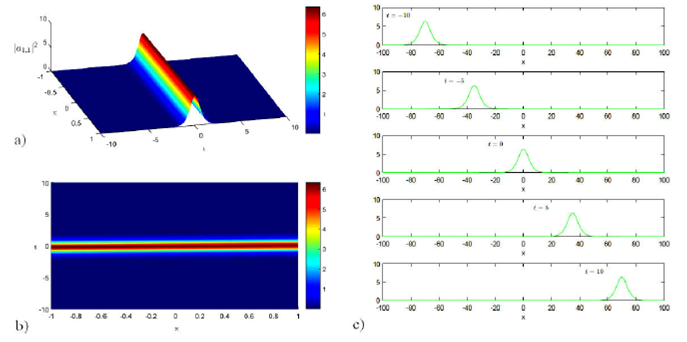
Figure 1 The plot of the bright soliton of |a 1;1 |2 of the solution Eq. (32) at A1 = 1, C2 = 0:019, C4 = -0:3, v = 7. 

Figure 2 The plot of dark soliton of |a 1;1 |2 of the solution Eq. (33) at A1 = 1, C0 = 520:62, C2 = -58:91, C4 = 1:66; v = 0:3. 

3.3.The Sine-Gordon expansion approach

Plugging the predicted solution (27) and its necessary derivatives into (9), we get an over-determined system containing the combination of cos(ω) and sin(ω). Setting the same powers of sini(ω)cosj(ω) equal to zero, a system of algebraic equations is deduced. Solving this system, we report the following result:

Set 1:

A0=B1=0, A1=c+2v2k12+c2-4vk1+22γ,   β2=c+2v2k12+c2-4vk1+22v2 (50)

Figure 3 The plot of dark soliton |a 1;1 |2 of the solution Eq. (33) at A1 = 1:5, C0 = 0:5, C4 = 0:5, v = 4:5, a) [C2 = -0:25;C2 = -0:5;C2 = -0:75]; b) [C2 = -1:25;C2 = -1:50;C2 = -1:75] respectively. 

Then, the solutions of (2) corresponding to (50) are

a4,1(x,t)=A1tanh(x-vt)eif(x-vt), (51)

a4,2(x,t)=A1coth(x-vt)eif(x-vt), (52)

where (51) and (52) represent dark optical and singular soliton solutions, respectively.

Furthermore, (33) is read like (51) under the constraint conditions C2 = -1, and C4 = 1/2 (3). On the other side when C2-1, (33) and (51) (dark-solitons) have the same form, but differ in width and amplitude during long distance communication taking advantage of its stability under the influence of the material losses (see 4). So, it is important to conserve the obtained two results.

Set 2:

A0=A1=0,  B1=γc2-(vk1-1)2+cγ,  β2=-c2-(vk1-1)2+cv2. (53)

Then, the solutions of (2) corresponding to (53) are

a5,1(x,t)=B1sech(x-vt)eif(x-vt), (54)

a5,2(x,t)=iB1csch(x-vt)eif(x-vt), (55)

where (54) and (55) represent bright optical and singular soliton solutions, respectively.

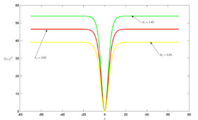
Figure 4 The plot of dark soliton |a 1;2 |2 of the solution Eq. (33) at [A1 = 1:5, C0 = 51:62, C2 = -2:31, C4 = 0:26, c = 1:2, v = 0:15, γ = 0:35, β2 = 1, k1 = 1:65], [A1 = 1:5, C0 = 38:43, C2 = -2:002, C4 = 0:026, c = 1:2, v = 0:15, γ = 0:35, β2 = 1, k2 = 2:65], [A1 = 1:5, C0 = 27:18, C2 = -1:68, C4 = 0:026, c = 1:2, v = 0:15, γ = 0:35, β2 = 1, k1 = 3:65] respectively. 

Remark: By integrating from (4) with along to (7), we have

f(ξ)=(1-k1v)β2v2dξ+ξ0, (56)

where ξ0 is an integration constant. However when k1 = 0, which corresponds to the conventional two-core fiber design 21, the chirp obtained depends only with the GVD and the speed of the soliton.

4.Conclusion

In this paper, we have investigated solitary waves for two-core optical fiber with coupling-coefficient dispersion and Kerr nonlinearity. It have been constructed an exact analytical soliton-like solutions by utilizing the traveling-wave hypothesis and hence the constraint relation fall out by adopting three integration techniques. By adopting the modified auxiliary equation and the sine-Gordon expansion approch, we obtain solitary waves; additionally, trigonometric function solutions and rational function solutions also emerge. Moreover, some new solitons solutions have been obtained, among which Eqs. (35)-(37), (40), (41), (43), (44), (49), and (55) are not reported in the standard integration method results summarized in of Ref. 30. The righteousness of the auxiliary equation method in this work is that, without a lot convoluted calculations, we obtain bright, dark and W-shape bright solitons. Thus, it is also important to note that the auxiliary equation method is independent of the integrability of the nonlinear differential equation (9). The obtained results will certainly have an important effect in nonlinear optical fibers in the field of solitary waves and can be helpful in describing communication systems ans ultra fast phenomena.

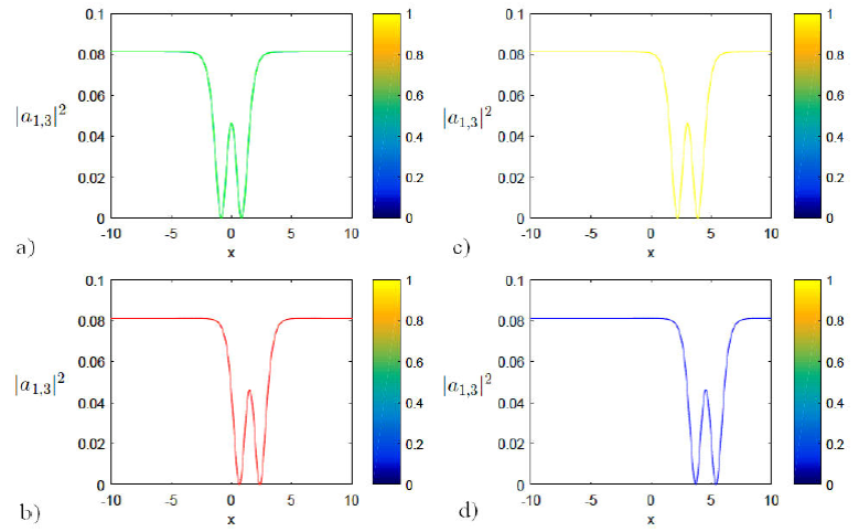
Figure 5 The plot of W-shape bright soliton |a 1;3 |2 of the solution Eq. (35) at a) [k1 = 0:975; c = 0:0461; v = 1:981; γ = 1:98005;A1 = 0:71; β2 = :90; t = 0], b) [k1 = 0:975; c = 0:0461; v = 1:981; γ = 1:98005;A1 = 0:71; β2 = :90; t = 3], c) [k1 = 0:975; c = 0:0461; v = 1:981; γ = 1:98005;A1 = 0:71; β2 = :90; t = 6], d) [k1 = 0:975; c = 0:0461; v = 1:981; γ = 1:98005;A1 = 0:71; β2 = :90; t = 9] respectively. 

References

1. G. Meltz, J. R. Dunphy, W. W. Morey, and E. Snitzer, Crosstalk fiber-optic temperature sensor, Appl. Opt. 22 (1983) 464, https://doi.org/10.1364/AO.22.000464. [ Links ]

2. Y. V. Kartashov, V. A. Vysloukh, and L. Torner, Soliton Shape and Mobility Control in Optical Lattices, Prog. Opt. 52 (2009) 63, https://doi.org/10.1016/S0079-6638(08)00004-8. [ Links ]

3. M. Arshad, A. R. Seadawy, and D. Lu, Bright-dark solitary wave solutions of generalized higher-order nonlinear Schrödinger equation and its applications in optics, J. Electromagn. Waves Appl. 31 (2017) 1711, https://doi.org/10.1080/09205071.2017.1362361. [ Links ]

4. P. G. Kevrekidis and D. J. Frantzeskakis, Solitons in coupled nonlinear Schrödinger models: A survey of recent developments, Rev. Phys. 1 (2016) 140, https://doi.org/10.1016/j.revip.2016.07.002. [ Links ]

5. A. Biswas, Soliton solutions of the perturbed resonant nonlinear Schrödinger’s equation with full nonlinearity by semiinverse variational principle. Quantum Phys. Lett. 1 (2013) 79. [ Links ]

6. M. Liu and P. Shum, Generalized coupled nonlinear equations for the analysis of asymmetric two-core fiber coupler, Opt. Express 11 (2003) 116, https://doi.org/10.1364/OE.11.000116. [ Links ]

7. B. A. Malomed, I. M. Skinner, and R. S. Tasgal, Solitons in a nonlinear optical coupler in the presence of the Raman effect, Opt. Commun. 139 (1997) 247, https://doi.org/10.1016/S0030-4018(97)00117-X. [ Links ]

8. M. S. Osman et al., The unified method for conformable time fractional Schrödinger equation with perturbation terms, Chin. J. Phys. 56 (2018) 2500, https://doi.org/10.1016/j.cjph.2018.06.009. [ Links ]

9. M. S. Osman, H. Rezazadeh, M. Eslami, A. Neirameh, and M. Mirzazadeh, Analytical study of solitons to Benjamin-Bona-Mahony-Peregrine equation with power law nonlinearity by using three methods, UPB Sci. Bull. A 80 (2018) 267. [ Links ]

10. M. Hesami et al., Generation of bright spatial quasi-solitons by arbitrary initial beam profiles in local and nonlocal (1+1)-Dimensional nonlinear media, Optik 202 (2020) 163504, https://doi.org/10.1016/j.ijleo.2019.163504. [ Links ]

11. A. Biswas et al., Resonant optical solitions with dualpower law nonlinearity and fractional temporal evolution, Optik 165 (2018) 233, https://doi.org/10.1016/j.ijleo.2018.03.123. [ Links ]

12. M. Hesami, M. Avazpour, and M. M. Méndez Otero, Transforming higher order bright and dark solitons to the first order solitons in Kerr medium: A review, Optik 202 (2020) 163695, https://doi.org/10.1016/j.ijleo.2019.163695. [ Links ]

13. M. Eslami, H. Rezazadeh, M. Rezazadeh, and S. S. Mosavi, Exact solutions to the space-time fractional Schrödinger-Hirota equation and the space-time modified KDV Zakharov-Kuznetsov equation, Opt. Quantum Electron. 49 (2017) 279, https://doi.org/10.1007/s11082-017-1112-6. [ Links ]

14. H. Rezazadeh, New solitons solutions of the complex Ginzburg-Landau equation with Kerr law nonlinearity, Optik 167 (2018) 218, https://doi.org/10.1016/j.ijleo.2018.04.026. [ Links ]

15. H. Rezazadeh, H. Tariq, M. Eslami, M. Mirzazadeh, and Q. Zhou, New exact solutions of nonlinear conformable time-fractional Phi-4 equation, Chin. J. Phys. 56 (2018) 2805, https://doi.org/10.1016/j.cjph.2018.08.001. [ Links ]

16. L.-C. Zhao, S.-C. Li, and L. Ling, Rational W-shaped solitons on a continuous-wave background in the Sasa-Satsuma equation, Phys. Rev. E 89 (2014) 023210, https://doi.org/10.1103/PhysRevE.89.023210. [ Links ]

17. A.W. Snyder, Coupled-Mode Theory for Optical Fibers, J. Opt. Soc. Am. 62 (1972) 1267, https://doi.org/10.1364/JOSA.62.001267. [ Links ]

18. S. Shamseldeen, M. S. A. Latif, A. Hamed, and H. Nour, New soliton solutions in dualcore optical fibers, Commun. Math. Model. Appl. 2 (2017) 39. [ Links ]

19. Z. Wang et al., Coupling in dual-core photonic bandgap fibers: theory and experiment, Opt. Express 15 (2007) 4795, https://doi.org/10.1364/OE.15.004795. [ Links ]

20. T. S. Raju, P. K. Panigrahi, and K. Porsezian, Nonlinear compression of solitary waves in asymmetric twin-core fibers, Phys. Rev. E 71 (2005) 026608, https://doi.org/10.1103/PhysRevE.71.026608. [ Links ]

21. M. Younis, S. T. R. Rizvi, Q. Zhou, A. Biswas, and M. Belic, Optical solitons in dual-core fibers with G’/G-expansion scheme, J. Optoelectron. Adv. Mater. 17 (2015) 505. [ Links ]

22. J. Zhang and C. Dai, Bright and dark optical solitons in the nonlinear Schrödinger equation with fourth-order dispersion and cubic-quintic nonlinearity, Chin. Opt. Lett. 3 (2005) 295. [ Links ]

23. H. Alphonse et al., Optical solitons for higher-order nonlinear Schrödinger equation with three exotic integration architectures, Optik 179 (2019) 861, https://doi.org/10.1016/j.ijleo.2018.11.027. [ Links ]

24. M. M. A. Khater, R. A. M. Attia, and D. Lu, Modified Auxiliary Equation Method versus Three Nonlinear Fractional Biological Models in Present ExplicitWave Solutions, Math. Comput. Appl. 24 (2019) 1, https://doi.org/10.3390/mca24010001. [ Links ]

25. R. A. M. Attia, D. Lu, and M. M. A. Khater, Chaos and Relativistic Energy-Momentum of the Nonlinear Time Fractional Duffing Equation, Math. Comput. Appl. 24 (2019) 10, https://doi.org/10.3390/mca24010010. [ Links ]

26. M. S. Osman, D. Lu, M. M. A. Khater, and R. A. M. Attia, Complex wave structures for abundant solutions related to the complex Ginzburg-Landau model, Optik 192 (2019) 162927, https://doi.org/10.1016/j.ijleo.2019.06.027. [ Links ]

27. C. Yan, A simple transformation for nonlinear waves, Phys. Lett. A 224 (1996) 77, https://doi.org/10.1016/S0375-9601(96)00770-0. [ Links ]

28. Z. Yan and H. Zhang, New explicit and exact travelling wave solutions for a system of variant Boussinesq equations in mathematical physics, Phys. Lett. A 252 (1999) 291, https://doi.org/10.1016/S0375-9601(98)00956-6. [ Links ]

29. L.-H. Zhang, Travelling wave solutions for the generalized Zakharov-Kuznetsov equation with higher-order nonlinear terms, Appl. Math. Comput. 208 (2009) 144, https://doi.org/10.1016/j.amc.2008.11.020. [ Links ]

Received: November 18, 2020; Accepted: December 01, 2020

Creative Commons License This is an open-access article distributed under the terms of the Creative Commons Attribution License