Solutions of generalized fractional perturbed Zakharov-Kuznetsov equation arising in a magnetized dusty plasma

Akinyemi, L.; Akinyemi, L.

doi:10.31349/revmexfis.67.060703

Servicios Personalizados

Revista

Articulo

Indicadores

Links relacionados

Otros
Otros

Permalink

Revista mexicana de física

versión impresa ISSN 0035-001X

Rev. mex. fis. vol.67 no.6 México nov./dic. 2021 Epub 14-Mar-2022

https://doi.org/10.31349/revmexfis.67.060703

Research

Gravitation, Mathematical Physics and Field Theory

Solutions of generalized fractional perturbed Zakharov-Kuznetsov equation arising in a magnetized dusty plasma

L. Akinyemi¹

^¹Department of Mathematics, Lafayette College, Easton, Pennsylvania, USA. e-mail: akinyeml@lafayette.edu

Abstract:

The generalized fractional perturbed (3+1) -dimensional Zakharov-Kuznetsov (PZK) equation, which appears in the magnetized two-ion-temperature dusty plasma, and quantum physics is considered. The sub-equation method in the conformable sense is proposed to obtain exact solutions to this equation. The new solutions obtained by the proposed method are dark soliton, multi-soliton, solitary wave, kink-shape, bell-shaped soliton, and periodic solutions that are substantial in the field of mathematical physics and can be of relevance in the field of plasma physics, also for future research.

Keywords: Perturbed (3 + 1)-dimensional Zakharov-Kuznetsov equation; conformable derivative; sub-equation method; Riccati equation; mathematical physics

PACS: 02.30.Jr; 47.35.Fg; 52.35.FP; 52.35.MW; 52.35.Sb

1.Introduction

The nonlinear evolution equations have played a fundamental role in the field of mathematical physics and many other areas of applied science. As an instance, in signal processing, dusty plasma, fluid dynamics, nonlinear optics, quantum mechanics, biology, and so forth (1)-(6). Examining the exact solutions of these nonlinear models help us to understand the mechanism, application and gives better knowledge of the model. With the virtue of these solutions, a better vision can be captured into the physical feature of the considered model. In recent years, series of methods have been developed to obtain the exact and approximate solutions of the nonlinear evolution equations in mathematical physics, as an instance, the Jacobi elliptic function method ⁷, Adomian decomposition method ⁸, sine-cosine method ⁹^,¹⁰, first integral method ¹¹^,¹², variational iteration method ¹³^,¹⁴, extended tanh method ¹⁵^,¹⁶, q-homotopy analysis method ¹⁷^-¹⁹, exp-function method²⁰^-²², q-homotopy analysis transform method ²³^-²⁵, tanh-sech method ²⁶^,²⁷, homotopy perturbation method (28), (G´/G)-expansion method ²⁹^,³⁰, fractional reduced differential transform method ³¹^,³², homogeneous balance method ³³^,³⁴, inverse scattering method ³⁵, iterative shehu transform method ³⁶, homotopy analysis method ³⁷^,³⁸, Jacobi elliptic expansion method ³⁹^,⁴⁰, residual power series method ⁴¹^-⁴³, perturbation-iteration algorithm ⁴⁴^,⁴⁵, modified Kudryashov method (46), new extended direct algebraic method ⁴⁷, Sardar sub-equation method ⁴⁸, Sine-cosine and sinh-cosh techniques ⁴⁹, simple equation method ⁵⁰ and so on.

The (3+ 1) -dimensional Zakharov-Kuznetsov (ZK) equation which comprises of the nonlinear term “PP _x ”and third-order dispersion term “P_xxx ” is restricted to the waves of small amplitudes only is presented by

$Δ:=Pt+A PPx+B Pxxx+C(Pxyy+Pxzz)=0,$ (1)

where P represents electrostatic potential, the physical quantities A, B and C are constants. Seadawy et al. ⁵¹^,⁵² and Zhen et al. ⁵³ have outlined these physical quantities. The width of the soliton and its velocity deviate from the predictions of this equation when the amplitude of the wave increases. As a result, an additional fifth-order dispersion term which is a higher-order dispersion term, $‘‘EPxxxxx",$ is added to (1) to overcome this problem (see ⁵¹^-⁵⁴, for more detailed). The new perturbed -(3+1)dimensional ZK equation reads

$Δ:=Pt+APPx+BPxxx\na+C(Pxyy+Pxzz)+EPxxxxx=0.$ (2)

In this present study, our objective is to further complement the previous studies conducted on the perturbed (3+1)-dimensional ZK equation by introducing the more general form by replacing the nonlinear term “PP _x” with $‘‘PkPx".$ We now consider the generalized fractional form of this equation as

$DtγγP+APkPx+BPxxx+C(Pxyy+Pxzz)+EPxxxxx=0,0<γ≤1,t>0,$ (3)

where k is a positive number, γ is the fractional-order and $E$ is a smallness parameter. For this purpose, we have carefully proposed the sub-equation method of conformable type to find analytic closed-form solutions of (3). The solutions consist of the dark soliton, multi-soliton, kink-shape, solitary wave, bell-shaped solitons, and periodic solutions, which are all substantial in the field of mathematical physics. When $γ=1, k=1,$ and $E=0,$ (3) reduces to the standard Zakharov?Kuznetsov (ZK) equation (see (1). For γ = 1, k = 2 and $E=0,$ (3) reduces to the modified KdV-ZK equation developed for a plasma comprised of cool and hot electrons and a species of fluid ions ⁵⁵. The case when k = 1,2 and 4 are considered in this present study. It is worth mentioning that the case when γ = 1 and k = 1 in (3) have been investigated by the following authors. Elwakil et al. in ⁵⁶ have studied the electron-acoustic solitary waves in a magnetized collisionless plasma consisting of a cold electron fluid and non-thermal hot electrons obeying a non-thermal distribution, and stationary. Ali et al. in ⁵⁷ have investigated the exact solutions by using a sine-cosine method and modified Kudryashov methods and constructed six Lie point symmetries and nonlocal conservation laws for this equation. Recently, in ⁵⁸, using two methods, Lie symmetry analysis and generalized exponential rational function. The authors present new exact solutions through optimal systems of one-dimensional Lie subalgebras; some solitary waves depict single soliton, multi-soliton, and annihilation profiles and six other closed-form solutions. To our knowledge, the case when k = 2 and k = 4 have not been studied before.

The rest of the paper is organized as follows: Section 2 gives a brief discussion of conformable derivatives which includes the definitions, basic properties, lemmas, and theorems. Section 3 presents the general idea of the sub-equation method. In 4, the application of sub-equation to time-fractional perturbed (3+1)-dimensional ZK equation of conformable type is demonstrated. In 5, the graphical representation of some solutions is depicted in 3D for different fractional orders. Finally, 6 gives the conclusion.

2.Preliminaries

This section contains a brief discussion of conformable derivatives, which includes the definitions, basic properties, lemmas, and theorems. Most of the concepts presented in this section have been introduced in ⁵⁹^,⁶⁰

Definition 2.1. Let $P:[0,∞)→R.$ The conformable derivative of P of order γ is given by

$DγP(t)=limε→0P(t+εt1-γ)-P(t)ε,∀t>0,γ∈(0,1).$ (4)

Furthermore, If P is γ-differentiable in some interval $(0,ζ)$ where $ζ>0,$ and $limt→0P(γ)(t)$ exists. We define

$P(γ)(0)=limt→0+P(γ)(t).$ (5)

Lemma 2.2.⁵⁹Let $γ∈(0,1]$ and P, Q be γ-differentiable at a point t > 0. Then

$Dγ(δ1P+δ2Q)=δ1DγP+δ2DγQ,∀δ1,δ2∈R$ .
$Dγ(tσ)=σtσ-γ,∀σ∈R$ .
$Dγ(PQ)=PDγQ+QDγP$ .
$Dγ(PQ)=QDγP-PDγQQ2,$ provided $Q≠0$ .
$Dγ(C)=0,$ where C is a constant.

Lemma 2.3.⁵⁹Let P be a differentiable and γ-differentiable function. Then

$DγP(t)=t1-γ∂P(t)∂t.$ (6)

Theorem 2.4.⁶¹^,⁶²Let $P:(0,∞)→R$ be a differentiable and γ-differentiable function. Let Q be a differentiable function defined in the range of P. Then

$Dtγ(P∘Q)(t)=t1-γQ(t)γ-1×Q'(t)Dtγ(P(Φ))|{Φ=Q(t)}.$ (7)

3.Algorithm of the proposed method

The main concept of the sub-equation method ⁶³^,⁶⁴ for solving FPDEs is presented below:

$F(P,Px,Py,Pz,Pxx,Pyy,Pzz,⋯,DtγP)=0.$ (8)

Here, $Dtγ$ is defined according to 2 with fractional order γ and an unknown function $P=P(x,y,z,t).$

Step. 1: Let $P(x,y,z,t)=P(ξ), ξ=px+qy+rz+s tγγ,$ where p, q, r and s are constants to be calculated respectively. With the help of the chain rule, we can transform Eq. (8) to an integer order nonlinear ODE given as

$G(P(ξ),P'(ξ),P''(ξ),P'''(ξ),⋯)=0.$ (9)

Step 2: We suppose that (9) has the solution:

$P(ξ)=e0+∑j=1Nejϑj(ξ), eN≠0,$ (10)

where p,q,r,s and $ej(j=0,1,⋯,N),$ are constants to be obtained accordingly. Balancing the highest-order derivative and biggest nonlinear term in Eq.(9) provides value for the integer N. The function $ϑ(ξ)$ satisfies the Riccati equation:

$ϑ'(ξ)=σ+ϑ2(ξ),$ (11)

where σ is a constant and the solutions are given as

$ϑ(ξ)={--σtanh⁡(-σξ),σ<0,--σcoth⁡(-σξ),σ<0,σtan⁡(σξ),σ>0,-σcot⁡(σξ),σ>0,-1ξ+ϕ,ϕ is a constant, σ=0.$ (12)

Step 3: Substituting Eqs. (10) and (11) into Eq.(9), we have some polynomial in $ϑj(ξ), (j=0,1,2⋯).$ Furthermore, setting the coefficients of $ϑj(ξ)$ to zero, results set of nonlinear algebraic equations in p,q,r,s and $ej(j=0,1,⋯,N).$

Step 4: Finally, by solving the equations found in Step 3. Then, substitute these constants p,q,r,s,σ and e_j into Eq.(10) in addition to Eq. (12), we conclude the desirable solutions for Eq. (8) immediately.

4.Sub-Equation Method to PZK Equations of Comformable Type

Here, the application of the sub-equation method to the time-fractional perturbed (3 + 1) -dimensional ZK equation of conformable type is presented. Consider

$DtγP+APkPx+BPxxx+C(Pxyy+Pxzz)+EPxxxxx=0.$ (13)

Application of chain rule on $P(x,y,z,t)=P(ξ), ξ=px+qy+rz+stγγ$ reduces Eq. (13) to a nonlinear ODE given as

$(s+pAPk)P'+(p3B+C(p q2+p r2))P'''+p5E P'''''=0.$ (14)

Balance principle to the terms $PkP'$ and $P'''''$ yields $N=4k.$ To obtain closed-form solutions, N must be an integer; therefore, we choose k = 1,2 and 4.

4.1.Solutions for k = 1:

For k = 1, we have N = 4, then Eq.(10) gives

$P(ξ)=e0+e1ϑ(ξ)+e2ϑ2(ξ)+e3ϑ3(ξ)+e4ϑ4(ξ).$ (15)

By substituting Eqs. (11) and (15) into Eq.(14), then equating the coefficients of $ϑr(ξ)$ to zero yields

$ϑ0(ξ):Ae0e1pσ+6e3σ3Bp3+Cpq2+Cpr2+2e1σ2Bp3+Cpq2+Cpr2+ 120Ee3p5σ4+16Ee1p5σ3+e1sσ=0,ϑ1(ξ):Ae12pσ+2Ae0e2pσ+24e4σ3Bp3+Cpq2+Cpr2+ 16e2σ2Bp3+Cpq2+Cpr2+960Ee4p5σ4+272Ee2p5σ3+2e2sσ=0, ϑ2(ξ):3Ae1e2pσ+3Ae0e3pσ+Ae0e1p+60e3σ2Bp3+Cpq2+Cpr2+ 8e1σBp3+Cpq2+Cpr2+1848Ee3p5σ3+136Ee1p5σ2+3e3sσ+e1s=0, ϑ3(ξ):2Ae22pσ+4Ae1e3pσ+4Ae0e4pσ+Ae12p+2Ae0e2p+ 152e4σ2(Bp3+Cpq2+Cpr2)+40e2σ(Bp3+Cpq2+Cpr2)+ 7744Ee4p5σ3+1232Ee2p5σ2+4e4sσ+2e2s=0,ϑ4(ξ):5Ae2e3pσ+5Ae1e4pσ+3Ae1e2p+3Ae0e3p+114e3σBp3+Cpq2+Cpr2+ 6e1Bp3+Cpq2+Cpr2+5808Ee3p5σ2+240Ee1p5σ+3e3s=0, ϑ5(ξ):3Ae32pσ+6Ae2e4pσ+2Ae22p+4Ae1e3p+4Ae0e4p+248e4σ(Bp3+Cpq2+Cpr2)+ 24e2(Bp3+Cpq2+Cpr2)+19264Ee4p5σ2+1680Ee2p5σ+4e4s=0,ϑ6(ξ):7Ae3e4pσ+5Ae2e3p+5Ae1e4p+60e3(Bp3+Cpq2+Cpr2)+6600Ee3p5σ+120Ee1p5=0,ϑ7(ξ):4Ae42pσ+3Ae32p+6Ae2e4p+120e4(Bp3+Cpq2+Cpr2)+19200Ee4p5σ+720Ee2p5=0,ϑ8(ξ):7Ae3e4p+2520Ee3p5=0,ϑ9(ξ):4Ae42p+6720Ee4p5=0.$ (16)

With the aid of Mathematica, we solve the above equations as

Case 1.

$e0=e0,e1=0,e2=-3360Ep4σA,e3=0,e4=-1680Ep4A,s=-Ae0p-1104Ep5σ2,r=±-Bp2-Cq2+52Ep4σC.$ (17)

By substituting Eq.(17) into Eq.(15) with solutions defined in Eq.(12), we have the required solutions of Eq.(13) as:

$P1=e0+3360Ep4σ2Atanh2(-σ&#091;px+qy+rz+sγtγ&#093;)-1680Ep4σ2Atanh4(-σ&#091;px+qy+rz+sγtγ&#093;), σ>0,P2=e0+3360Ep4σ2Acoth2(-σ&#091;px+qy+rz+sγtγ&#093;)-1680Ep4σ2Acoth4(-σ&#091;px+qy+rz+sγtγ&#093;), σ>0,P3=e0-3360Ep4σ2Atan2(σ&#091;px+qy+rz+sγtγ&#093;)-1680Ep4σ2Atan4(σ&#091;px+qy+rz+sγtγ&#093;), σ<0,P4=e0-3360Ep4σ2Acot2(σ&#091;px+qy+rz+sγtγ&#093;)-1680Ep4σ2Acot4(σ&#091;px+qy+rz+sγtγ&#093;), σ<0,P5=e0-1680Ep4Apx+qy±-Bp2-Cq2Cz-Ae0pγtγ+ϕ4, σ=0,$

where $ϕ$ is a constant, $s=-Ae0p-1104Ep5σ2$ and $r=±(-Bp2-Cq2+52Ep4σ)/C.$

Case 2.

$e0=e0,e1=0,e2=1680i(31Ep4σ+31iEp4σ)31A,e3=0,e4=-1680Ep4A,s=131(-31Ae0p-3720Ep5σ2+1368i31Ep5σ2),r=±-Bp2C-26Ep4σC-78iEp4σ31C-q2.$ (18)

The required solutions for Eq.(13) are

$P6=e0-1680iσ31Ep4σ+31iEp4σ31Atanh2(-σ[px+qy+rz+sγtγ])-1680Ep4σ2Atanh4(-σ[px+qy+rz+sγtγ]), σ<0,P7=e0-1680iσ31Ep4σ+31iEp4σ31Acoth2(-σ[px+qy+rz+sγtγ])-1680Ep4σ2Acoth4(-σ[px+qy+rz+sγtγ]), σ<0,P8=e0+1680iσ31Ep4σ+31iEp4σ31Atan2(σ[px+qy+rz+sγtγ])-1680Ep4σ2Atan4(σ[px+qy+rz+sγtγ]), σ>0,P9=e0+1680iσ31Ep4σ+31iEp4σ31Acot2(σ[px+qy+rz+sγtγ])-1680Ep4σ2Acot4(σ[px+qy+rz+sγtγ]), σ>0,P10=e0-1680Ep4Apx+qy±z-Bp2C-q2-Ae0pγtγ+ϕ4, σ=0,$

where $s=131-31Ae0p-3720Ep5σ2+1368i31Ep5σ2$ and $r=±-Bp2C-26Ep4σC-78iEp4σ31C-q2.$

Case 3.

$e0=e0,e1=0,e2=-1680i(31Ep4σ-31iEp4σ)31A,e3=0,e4=-1680Ep4A,s=131(-31Ae0p-1368i31Ep5σ2-3720Ep5σ2),r=±-Bp2C+78iEp4σ31C-26Ep4σC-q2.$ (19)

The required solutions for Eq.(13) are

$P11=e0+1680iσ31Ep4σ-31iEp4σ31Atanh2(-σ[px+qy+rz+sγtγ])-1680Ep4σ2Atanh4(-σ[px+qy+rz+sγtγ]), σ<0,P12=e0+1680iσ31Ep4σ-31iEp4σ31Acoth2(-σ[px+qy+rz+sγtγ])-1680Ep4σ2Acoth4(-σ[px+qy+rz+sγtγ]), σ<0,P13=e0-1680iσ31Ep4σ-31iEp4σ31Atan2(σ[px+qy+rz+sγtγ])-1680Ep4σ2Atan4(σ[px+qy+rz+sγtγ]), σ>0,P14=e0-1680iσ31Ep4σ-31iEp4σ31Acot2(σ[px+qy+rz+sγtγ])-1680Ep4σ2Acot4(σ[px+qy+rz+sγtγ]), σ>0,P15=e0-1680Ep4Apx+qy±z-Bp2C-q2-Ae0pγtγ+ϕ4, σ=0,$

where $s=131-31Ae0p-1368i31Ep5σ2-3720Ep5σ2$ and $r=±-Bp2C+78iEp4σ31C-26Ep4σC-q2.$

4.2.Solutions for k= 2:

When k = 2 we have N = 2 then Eq.(10) gives

$P(ξ)=e0+e1ϑ(ξ)+e1ϑ2(ξ).$ (20)

By substituting Eqs. (20) and (11) into (14), then equating the coefficients of ECUACION to zero yields

$ϑ0(ξ):Ae02e1pσ+2e1σ2(Bp3+Cpq2+Cpr2)+16Ee1p5σ3+e1sσ=0,ϑ1(ξ):2Ae0e12pσ+2Ae02e2pσ+16e2σ2(Bp3+Cpq2+Cpr2)+272Ee2p5σ3+2e2sσ=0,ϑ2(ξ):Ae13pσ+6Ae0e1e2pσ+Ae02e1p+8e1σ(Bp3+Cpq2+Cpr2)+136Ee1p5σ2+e1s=0,ϑ3(ξ):4Ae0e22pσ+4Ae12e2pσ+2Ae0e12p+2Ae02e2p+ 40e2σ(Bp3+Cpq2+Cpr2)+1232Ee2p5σ2+2e2s=0,ϑ4(ξ):5Ae1e22pσ+Ae13p+6Ae0e1e2p+6e1(Bp3+Cpq2+Cpr2)+240Ee1p5σ=0,ϑ5(ξ):2Ae23pσ+4Ae0e22p+4Ae12e2p+24e2(Bp3+Cpq2+Cpr2)+1680Ee2p5σ=0,ϑ6(ξ):5Ae1e22p+120Ee1p5=0,ϑ7(ξ):2Ae23p+720Ee2p5=0.$ (21)

With the help of Mathematica, we solve the above equations as

Case 1.

$e0=e0,\qe1=0,e2=-6ip210EA,s=-8i10AEe0p3σ-Ae02p+184Ep5σ2,r=±i10AEe0p2-Bp2-Cq2-40Ep4σC.$ (22)

By substituting Eq.(22) into Eq.(20) and using the solutions defined in Eq.(12), we obtain the required solutions to Eq.(13) as:

$P16=e0+6ip2σ10EAtanh2(-σ(px+qy+rz+sγtγ)), σ<0,P17=e0+6ip2σ10EAcoth2(-σ(px+qy+rz+sγtγ)), σ<0,P18=e0-6ip2σ10EAtan2(σ(px+qy+rz+sγtγ)), σ>0,P19=e0-6ip2σ10EAcot2(σ(px+qy+rz+sγtγ)), σ>0,P20=e0-6ip210EApx+qy±i10AEe0p2-Bp2-Cq2Cz-Ae02pγtγ+ϕ2, σ=0,$

where $s=-8i10AEe0p3σ-Ae02p+184Ep5σ2$ and $r=±i10AEe0p2-Bp2-Cq2-40Ep4σC.$

Case 2.

$e0=e0,\qe1=0,\qe2=6ip210EA,s=8i10AEe0p3σ-Ae02p+184Ep5σ2,r=±-i10AEe0p2-Bp2-Cq2-40Ep4σC.$ (23)

By substituting Eq.(23) into Eq.(20) and using the solutions defined in Eq.(12), we obtain the required solutions to Eq.(13) as:

$P21=e0-6ip2σ10EAtanh2(-σ(px+qy+rz+stγγ)), σ<0,P22=e0-6ip2σ10EAcoth2(-σ(px+qy+rz+stγγ)), σ<0,P23=e0+6ip2σ10EAtan2(σ(px+qy+rz+stγγ)), σ>0,P24=e0+6ip2σ10EAcot2(σ(px+qy+rz+stγγ)), σ>0,P25=e0+6ip210EApx+qy±-i10AEe0p2-Bp2-Cq2Cz-Ae02pγtγ+ϕ2, σ=0,$

where $s=8i10AEe0p3σ-Ae02p+184Ep5σ2$ and $r=±-i10AEe0p2-Bp2-Cq2-40Ep4σC.$

4.3.Solutions for k= 4:

When k = 4 we have N = 1, then Eq.(10) yields

$P(ξ)=e0+e1ϑ(ξ).$ (24)

By substituting Eqs. (24) and (11) into Eq.(14), then equating the coefficients of $ϑr(ξ)$ to zero gives

$ϑ0(ξ):Ae04e1pσ+2e1σ2Bp3+Cpq2+Cpr2+16Ee1p5σ3+e1sσ=0,ϑ1(ξ):4Ae03e12pσ=0,ϑ2(ξ):6Ae02e13pσ+Ae04e1p+8e1σBp3+Cpq2+Cpr2+136Ee1p5σ2+e1s=0,ϑ3(ξ):4Ae0e14pσ+4Ae03e12p=0,ϑ4(ξ):Ae15pσ+6Ae02e13p+6e1(Bp3+Cpq2+Cpr2)+240Ee1p5σ=0,ϑ5(ξ):4Ae0e14p=0,ϑ6(ξ):Ae15p+120Ee1p5=0.$ (25)

By utilizing Mathematica, we solve the above equations as

Case 1:

$e0=e0, e1=±(1+i)p30EA4,s=24Ep5σ2,r=±-Bp2-Cq2-20Ep4σC.$ (26)

By substituting Eq.(26) into Eq.(24) and using the solutions defined in Eq.(12), we obtain the required solutions to Eq.(13) as:

$P26=±(1+i)p-σ30EA4tanh⁡-σpx+qy±-Bp2-Cq2-20Ep4σCz+24Ep5σ2γtγ,σ<0,P27=±(1+i)p-σ30EA4coth⁡-σpx+qy±-Bp2-Cq2-20Ep4σCz+24Ep5σ2γtγ,σ<0,P28=∓(1+i)pσ30EA4tan⁡σpx+qy±-Bp2-Cq2-20Ep4σCz+24Ep5σ2γtγ,σ>0,P29=±(1+i)pσ30EA4cot⁡σpx+qy±-Bp2-Cq2-20Ep4σCz+24Ep5σ2γtγ,σ>0,P30=±(1+i)p30E4A4px+qy±-Bp2C-q2z+ϕ,σ=0.$

Case 2:

$e0=e0,e1=±(-1+i)p30EA4,s=24Ep5σ2,r=±-Bp2-Cq2-20Ep4σC.$ (27)

By substituting Eq.(27) into Eq.(24) and using the solutions defined in Eq.(12), we obtain the required solutions to Eq.(13) as:

$P31=±(-1+i)p-σ30EA4tanh⁡-σpx+qy±-Bp2-Cq2-20Ep4σCz+24Ep5σ2γtγ,σ<0,P32=±(-1+i)p-σ30EA4coth⁡-σpx+qy±-Bp2-Cq2-20Ep4σCz+24Ep5σ2γtγ,σ<0,P33=∓(-1+i)pσ30EA4tan⁡σpx+qy±-Bp2-Cq2-20Ep4σCz+24Ep5σ2γtγ,σ>0,P34=±(-1+i)pσ30EA4cot⁡σpx+qy±-Bp2-Cq2-20Ep4σCz+24Ep5σ2γtγ,σ>0,P35=±(-1+i)p30E4A4(px+qy±-Bp2C-q2z+ϕ),σ=0.$

5.Graphical representation of some solutions

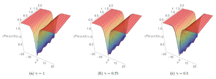
The absolute behavior in 3D plots with integer and fractional order respectively $γ=1, γ=0.75,$ and 0.5 are presented for some solutions in Fig.1-8. These plots reveal different structures such as the dark soliton, multi-soliton, solitary wave, bell-shaped soliton, periodic and kink-type solutions which give the readers a better vision of the behavior of these solutions and captured some physical features of the considered model. Furthermore, Fig.7 and 8 display the effect of adding a new perturbation term on the profile of the solution.

Figure 1 The plots of P₁ solution for A = 1; B = 2; C = -20; y = z = 2; E = 0:5; σ = -1; e₀ = 0:5; p = 0:2 and q = 0:2:

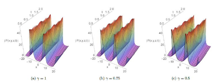
Figure 2 The plots of P₃ solution for A = 1; B = 2; C = -20; y = z = 2; E = 0:5; – = 1; e0 = 0:5; p = 0:2 and q = 0:2:

Figure 3 The plots of P₂₀ solution for A = 1; B = 2; C = -1; y = z = 2; E = 0:5; φ = 1; e0 = 3; p = 0:2 and q = 0:2:

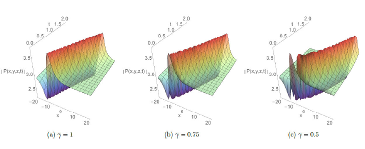
Figure 4 The plots of P₂₅ solution for A = 1; B = 2; C = -1; y = z = 2; E = 0:5; φ = 1; e₀ = 3; p = 0:2 and q = 0:2:

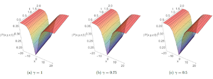
Figure 5 The plots of P₂₆ solution for A = 1; B = 2; C = 10; y = z = 2; E = 0:1; σ = -1; e₀ = 3; p = 0:2 and q = 0:2:

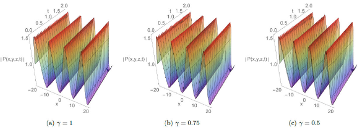
Figure 6 The plots of P₂₈ solution for A = 1; B = 2; C = 10; y = z = 2; E = 0:8; σ = 1; e₀ = 3; p = 0:3 and q = 0:3:

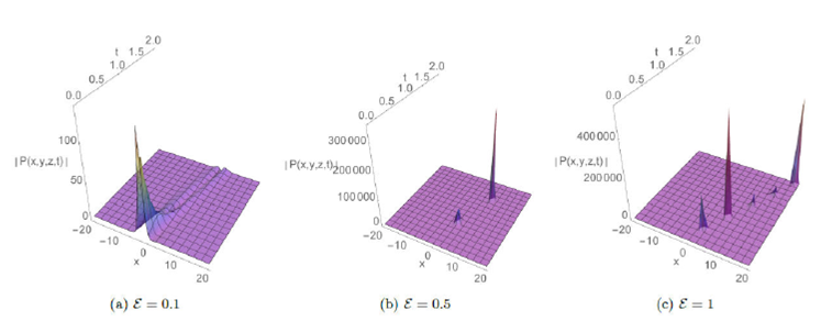
Figure 7 The effect of the parameter E on solution profile of P₁₁ for γ = 1; A = 1; B = 2; C = 10; y = z = 2; σ = -1; e₀ = 3; p = 0:5 and q = 0:5:

Figure 8 The effect of the parameter E on solution profile of P₁₆ for γ = 1; A = 1; B = 2; C = -5; y = z = 2; σ = -1; e₀ = 3; p = 0:5 and q = 0:5:

6.Conclusion

In this paper, we introduced the generalized time-fractional perturbed (3+1) Zakharov-Kuznetsov (PZK) equations which describe the nonlinear dust-ion-acoustic waves in the magnetized two-ion-temperature dusty plasmas. We investigate the exact solutions by the use the of sub-equation method in the conformable sense. The use of conformable derivative in this study gives flexibility when applying to the proposed model and satisfies the power rule, product rule, quotient rule, integration by parts, chain rule, linearity, and the derivatives with constant is zero. The newly obtained solutions by the proposed method are, respectively, the dark soliton multi-soliton, kink-shape, solitary wave, periodic and bell-shaped soliton solutions that are significant in the field of mathematical physics. Graphical representation (see Fig. 1 to 8) of obtained solutions are plotted in 3D for particular values of parameters. Figures 7 and 8, demonstrate the effect of adding a higher-order dispersion term $‘‘EPxxxxx"$ to Eq.(1). The performance of this method is reliable and effective and the obtained results are in a more general form. Finally, through Mathematica, we have authenticated the obtained solutions by substituting them back into the proposed equation.

References

1. L. Akinyemi, M. Senol, M. Mirzazadeh, and M. Eslami, Optical solitons for weakly nonlocal Schrödinger equation with parabolic law nonlinearity and external potential, Optik 230 (2021) 1, https://doi.org/10.1016/j.ijleo.2021.166281. [ Links ]

2. L. Akinyemi , M. Senol, and S. N. Husen, Modified homotopy methods for generalized fractional perturbed Zakharov-Kuznetsov equation in dusty plasma. Adv. Differ. Equ. 2021 (2021) 1, https://doi.org/10.1186/s13662-020-03208-5. [ Links ]

3. M. Mirzazadeh, L. Akinyemi, M. Senol, and K. Hosseini, A variety of solitons to the sixth-order dispersive (3 + 1)- dimensional nonlinear time-fractional Schrodinger equation with cubic-quintic-septic nonlinearities, Optik(2021) 166318, https://doi.org/10.1016/j.ijleo.2021.166318. [ Links ]

4. M.J. Ablowitz, Nonlinear DispersiveWaves: Asymptotic Analysis and Solitons, Cambridge University Press: Cambridge, (2011) [ Links ]

5. I. Owusu-Mensah, L. Akinyemi, B. Oduro, and O. S. Iyiola, A fractional order approach to modeling and simulations of the novel COVID-19. Adv. Differ. Equ. 2020 (2020) 1, https://doi.org/10.1186/s13662-020-03141-7. [ Links ]

6. A. Biswas et al., Optical solitons having weak non-local nonlinearity by two integration schemes, Optik. 164 (2018) 380. [ Links ]

7. Z. Yan, Abundant families of Jacobi elliptic function solutions of the (2 + 1)-dimensional integrable Davey-Stewartson-type equation via a new method. Chaos Soliton Fract. 18 (2003) 299, https://doi.org/10.1016/S0960-0779(02)00653-7. [ Links ]

8. G. Adomian, Solving Frontier Problems of Physics: The Decomposition Method. Kluwer, (1994). [ Links ]

9. A. M. Wazwaz, The sine-cosine method for obtaining solutions with compact and noncompact structures. Appl. Math. Comput. 159(2004) 559, https://doi.org/10.1016/j.amc.2003.08.136. [ Links ]

10. A. M. Wazwaz, A sine-cosine method for handling nonlinear wave equations. Math. Comput. Model. 40 (2004) 499, https://doi.org/10.1016/j.mcm.2003.12.010. [ Links ]

11. S. El-Ganaini, Solutions of some class of nonlinear PDEs in mathematical physics. J. Egypt. Math. Soc. 24 (2016) 214, http://dx.doi.org/10.1016/j.joems.2015.02.005. [ Links ]

12. S. I. A. El-Ganaini, Traveling wave solutions to the generalized Pochhammer-Chree (PC) equations using the first integral method Math. Probl. Eng. 2011 (2011) 1, doi:10.1155/2011/629760. [ Links ]

13. S. Das, Analytical solution of a fractional diffusion equation by variational iteration method. Comput. Math. Appl. 57 (2009) 483, https://doi.org/10.1016/j.camwa.2008.09.045. [ Links ]

14. J. H. He, Approximate analytical solution for seepage flow with fractional derivatives in porous media. Comput. Meth. Appl. Mech. Eng. 167 (1998) 57, https://doi.org/10.1016/S0045-7825(98)00108-X. [ Links ]

15. E. Fan, Extended tanh-function method and its applications to nonlinear equations. Phys. Lett. A 277 (2000) 212, https://doi.org/10.1016/S0375-9601(00)00725-8. [ Links ]

16. S. A. El-Wakil and M. A. Abdou, New exact travelling wave solutions using modified extended tanh-function method. Chaos Soliton Fract. 31(2007) 840, https://doi.org/10.1016/j.chaos.2005.10.032. [ Links ]

17. L. Akinyemi, q-Homotopy analysis method for solving the seventh-order time-fractional Lax’s Korteweg-de Vries and Sawada-Kotera equations. Comp. Appl. Math. 38 (2019) 1, https://doi.org/10.1007/s40314-019-0977-3. [ Links ]

18. L. Akinyemi , O.S. Iyiola, and U. Akpan, Iterative methods for solving fourth- and sixth order time-fractional Cahn-Hillard equation. Math. Meth. Appl. Sci. 43 (2020) 4050. https://doi.org/10.1002/mma.6173 [ Links ]

19. M.A. El-Tawil and S.N. Huseen, The Q-homotopy analysis method (q-HAM). Int. J. Appl. Math. Mech. 8 (2012) 51. [ Links ]

20. J.H., He and X.H. Wu, Exp-function method for nonlinear wave equations. Chaos Solitons Fract. 30 (2006) 700, https://doi.org/10.1016/j.chaos.2006.03.020. [ Links ]

21. E. Yusufoglu, New solitary solutions for the MBBM equations using Exp-function method. Phys. Letters A 372 (2008) 442, https://doi.org/10.1016/j.physleta.2007.07.062. [ Links ]

22. S. Zhang, Application of Exp-function method to highdimensional nonlinear evolution equation. Chaos, Solitons Fract. 38 (2008) 270, DOI: 10.1016/j.chaos.2006.11.014. [ Links ]

23. L. Akinyemi andS.N. Huseen , A powerful approach to study the new modified coupled Korteweg-de Vries system. Math. Comput. Simul. 177 (2020) 556, https://doi.org/10.1016/j.matcom.2020.05.021. [ Links ]

24. L. Akinyemi and O.S. Iyiola, A reliable technique to study nonlinear time-fractional coupled Korteweg-de Vries equations. Adv. Differ. Equ. 2020 (169) (2020) 1, https://doi.org/10.1186/s13662-020-02625-w. [ Links ]

25. D. Kumara, J. Singha, and D. Baleanu, A new analysis for fractional model of regularized long-wave equation arising in ion acoustic plasma waves. Math. Meth. Appl. Sci. 40 (2017) 5642. https://doi.org/10.1002/mma.4414. [ Links ]

26. W. Malflietand W. Hereman, The tanh method: I. Exact solutions of nonlinear evolution and wave equations. Phys. Scripta 54 (1996) 563, https://doi.org/10.1088/0031-8949/54/6/003. [ Links ]

27. A. M. Wazwaz , The tanh method for travelling wave solutions of nonlinear equations. Appl. Math. Comput. 154 (2004) 713, https://doi.org/10.1016/S0096-3003(03)00745-8. [ Links ]

28. J.H. He, Homotopy perturbation technique. Comput. Meth. Appl. Mech. Eng. 178 (1999) 257, http://dx.doi.org/10.1016/S0045-7825(99)00018-3. [ Links ]

29. M. Wang, X. Li, and J. Zhang, The G0 G -expansion method and travelling wave solutions of nonlinear evolution equations in mathematical physics. Phys. Letters A 372 (2008) 417, https://doi.org/10.1016/j.physleta.2007.07.051. [ Links ]

30. A. Bekir, Application of the G0 G -expansion method for nonlinear evolution equations. Phys. Letters A 372 (2008) 3400, https://doi.org/10.1016/j.physleta.2008.01.057. [ Links ]

31. Y. Keskin and G. Oturanc, Reduced differential transform method: a new approach to fractional partial differential equations. Nonlinear Sci. Lett. A 1 (2010) 61. [ Links ]

32. L. Akinyemi, A fractional analysis of Noyes-Field model for the nonlinear Belousov-Zhabotinsky reaction. Comp. Appl. Math. 39 (2020) 1, https://doi.org/10.1007/s40314-020-01212-9. [ Links ]

33. E.G. Fan and Q.H. Zhang, A note on the homogeneous balance method. Phys. Lett. A 246 (1998) 403, https://doi.org/10.1016/S0375-9601(98)00547-7. [ Links ]

34. M. L. Wang, Exact solutions for a compound KdV-Burgers equation. Phys. Lett. A 213 (1996) 279, https://doi.org/10.1016/0375-9601(96)00103-X. [ Links ]

35. V.O. Vakhnenko, E.J. Parkes, and A.J. Morrison, A Bäcklund transformation and the inverse scattering transform method for the generalised Vakhnenko equation. Chaos Soliton Fract. 17 (2003) 683, https://doi.org/10.1016/S0960-0779(02)00483-6. [ Links ]

36. L. Akinyemi and O.S. Iyiola, Exact and approximate solutions of time-fractional models arising from physics via Shehu transform. Math. Meth. Appl. Sci. (2020) 1, https://doi.org/10.1002/mma.6484. [ Links ]

37. S.J. Liao, On the homotopy analysis method for nonlinear problems. Appl. Math. Comput. 147 (2004) 499, https://doi.org/10.1016/S0096-3003(02)00790-7. [ Links ]

38. S. J. Liao, An approximate solution technique not depending on small parameters: a special example. Intern. J. Non-linear Mech. 30 (1995) 371, https://doi.org/10.1016/0020-7462(94)00054-E. [ Links ]

39. O. Tasbozan, Y. C¸ enesiz, and A. Kurt, New solutions for conformable fractional Boussinesq and combined KdV-mKdV equations using Jacobi elliptic function expansion method. The European Physical Journal Plus 131 (2016) 1, https://doi.org/10.1140/epjp/i2016-16244-x. [ Links ]

40. O. Tasbozan, A. Kurt, and A. Tozar, New optical solutions of complex Ginzburg-Landau equation arising in semiconductor lasers. Appl. Phys. B 125 (2019) 1, https://doi.org/10.1007/s00340-019-7217-9. [ Links ]

41. M. Alquran, K. Al-Khaled, and J. Chattopadhyay, Analytical solutions of fractional population diffusion model: residual power series. Nonlinear Studies 22(2015) 31. [ Links ]

42. M. Senol, O.S. Iyiola, H. Daei Kasmaei andL. Akinyemi , Efficient analytical techniques for solving time-fractional nonlinear coupled Jaulent-Miodek system with energy-dependent Schr¨odinger potential. Adv. Differ. Equ. 2019 (2019) 1, https://doi.org/10.1186/s13662-019-2397-5. [ Links ]

43. M. Senol , Analytical and approximate solutions of (2 + 1)-dimensional time-fractional Burgers-Kadomtsev-Petviashvili equation. Commun. Theor. Phys. 72 (2020) 1, https://doi.org/10.1088/1572-9494/ab7707. [ Links ]

44. M. Senol and I.T. Dolapci, On the Perturbation-Iteration Algorithm for fractional differential equations. Journal of King Saud University-Science 28 (2016) 69, https://doi.org/10.1016/j.jksus.2015.09.005. [ Links ]

45. M. Senol , S. Atpinar, Z. Zararsiz, S. Salahshour, and A. Ahmadian, Approximate solution of time-fractional fuzzy partial differential equations. Comput. Appl. Math. 38 (2019) 1, https://doi.org/10.1007/s40314-019-0796-6. [ Links ]

46. H. M. Srivastava et al., Traveling wave solutions to nonlinear directional couplers by modified Kudryashov method. Physica Scripta 95 (2020) 075217, https://doi.org/10.1088/1402-4896/ab95af. [ Links ]

47. H. Rezazadeh, New solitons solutions of the complex Ginzburg-Landau equation with Kerr law nonlinearity. Optik, 167 (2018) 218, https://doi.org/10.1016/j.ijleo.2018.04.026. [ Links ]

48. H. Rezazadeh, M. Inc and D. Baleanu, New Solitary Wave Solutions for Variants of (3+1)-DimensionalWazwaz-Benjamin-Bona-Mahony Equations. Frontiers in Physics, 8 (2020) 1, https://doi.org/10.3389/fphy.2020.00332. [ Links ]

49. J. Vahidi et al., New solitary wave solutions to the coupled Maccari’s system. Results in Physics, 21 (2021) 103801, https://doi.org/10.1016/j.rinp.2020.103801. [ Links ]

50. E. A. Az-Zo’bi et al., Abundant closed-form solitons for timefractional integro-differential equation in fluid dynamics. Opt Quant Electron 53 (2021) 132. https://doi.org/10.1007/s11082-021-02782-6 [ Links ]

51. A.R. Seadawy and D. Lu, Ion acoustic solitary wave solutions of three-dimensional nonlinear extended Zakharov-Kuznetsov dynamical equation in a magnetized two-ion-temperature dusty plasma. Results Phys. 6 (2016) 590, https://doi.org/10.1016/j.rinp.2016.08.023. [ Links ]

52. D. Lu, A.R. Seadawy , M. Arshad, and J. Wang, New solitary wave solutions of (3 + 1)-dimensional nonlinear extended Zakharov-Kuznetsov and modified KdV-Zakharov-Kuznetsov equations and their applications. Results Phys. 7 (2017) 899, https://doi.org/10.1016/j.rinp.2017.02.002. [ Links ]

53. H. Zhen, B. Tian, Y. Wang, W. Sun, and L. Liu, Soliton solutions and chaotic motion of the extended Zakharov-Kuznetsov equations in a magnetized two-ion-temperature dusty plasma. Phys Plasma 21 (2014) 073709, https://doi.org/10.1063/1.4885380. [ Links ]

54. S. Kumar and D. Kumar, Solitary wave solutions of (3 + 1)-dimensional extended Zakharov-Kuznetsov equation by Lie symmetry approach. Comput. Math. Appl. 77 (2019) 2096, https://doi.org/10.1016/j.camwa.2018.12.009. [ Links ]

55. R.L. Mace and M.A. Hellberg, The Korteweg-de Vries-Zakharov-Kuznetsov equation for electron-acoustic waves. Physics of Plasmas. 8 (2001) 2649, https://doi.org/10.1063/1.1363665. [ Links ]

56. S.A. Elwakil, E.K. El-Shewy, and H.G. Abdelwahed, Solution of the perturbed Zakharov-Kuznetsov (ZK) equation describing electron-acoustic solitary waves in a magnetized plasma. Chin. J. Phys. 49 (2011) 732. [ Links ]

57. M.N. Ali, A.R. Seadawy, and S.M. Husnine, Lie point symmetries exact solutions and conservation laws of perturbed Zakharov-Kuznetsov equation with higher-order dispersion term. Mod. Phys. Lett. A 34 (2019) 1950027, https://doi.org/10.1142/S0217732319500275. [ Links ]

58. D. Kumar and S. Kumar, Solitary wave solutions of PZK equation using lie point symmetries. Eur. Phys. J. Plus 135(2020) 1, https://doi.org/10.1140/epjp/s13360-020-00218-w. [ Links ]

59. R. Khalil, M. Al Horani, A. Yousef, and M. Sababheh, A new definition of fractional derivative. J. Comput. Appl. Math. 264 (2014) 65, https://doi.org/10.1016/j.cam.2014.01.002. [ Links ]

60. T. Abdeljawad, On conformable fractional calculus. J. Comput. Appl. Math. 279(2015) 57, https://doi.org/10.1016/j.cam.2014.10.016. [ Links ]

61. A. Atangana, D. Baleanu, and A. Alsaedi, New properties of conformable derivative. Open Math. 13 (2015) 889, DOI:10.1515/math-2015-0081. [ Links ]

62. M. Eslami, andH. Rezazadeh, The first integral method for Wu-Zhang system with conformable time-fractional derivative. Calcolo 53(2016) 475. [ Links ]

63. S. Zhang, and H.Q. Zhang, Fractional sub-equation method and its applications to nonlinear fractional PDEs. Phys. Lett. A 375 (2011) 1069, https://doi.org/10.1016/j.physleta.2011.01.029. [ Links ]

64. L. Akinyemi, M. Senol, and O.S. Iyiola, Exact solutions of the generalized multidimensional mathematical physics models via sub-equation method. Math. Comput. Simul. 182 (2021) 211. https://doi.org/10.1016/j.matcom.2020.10.017 [ Links ]

Received: December 16, 2020; Accepted: February 23, 2021

This is an open-access article distributed under the terms of the Creative Commons Attribution License