1 Introduction
Nowadays machine learning (ML) methods are mainly used to enhance solutions of specific problems in industry [1] and science [2]. In the last case, applications go from molecular design [3,4] to cosmology [5,6]. Particularly in condensed matter physics examples of ML developments are vast [7]. However, implementations of such methods to describe the liquid state are in the earliest stage, where problems like the determination of the molecular interaction potential from the microscopic structure [8] or the pattern identification in fluids [9] as well as the determination of transport properties [10] has been addressed.
On the other hand and in general terms, thermodynamic description of liquids can be done through experimental measurements of thermophysical properties like pressure, density, internal energy among other thermodynamic properties. However, since the time and cost needed to perform such experiments are high, just a subset of thermodynamic properties are able for measurement. Actually, results from such experiments can be consulted in different data banks for some specific molecular fluids [11,12]. Additionally, theoretical and computational approaches are commonly used to complement and in some cases predict the thermodynamic behaviour of liquids. In this regard, a correlation between the microscopic properties of the liquids and its macroscopical thermodynamic behaviour is always desirable.
The bridge between microscopic and macroscopic thermal properties is given by the equilibrium statistical mechanics, which provides a quite robust thermodynamic description of the liquid state [13]. This theoretical framework allows us to determine, for example, the fluid pressure, P, in terms of the microscopic structure, g(r) the interaction between molecules, u(r), density, ρ and temperature, T, of the liquid as [13]
where k is the Boltzmann constant. From Eq. (1) it is clear that if any of the macroscopic parameters, density or temperature, are unknown the pressure can not be determined.
Although from a theoretical or computational point of view a situation where density and temperature are both unknown is specially odd, there are some experimental systems of interest where the structure is easily determined but one or both thermodynamic variables are missing, for instance, in order to theoretically describe some non-vibrated granular systems it is fundamental to establish an effective temperature [14,15]. On the other hand, in temperature-dependent colloidal systems, like PNIPAM colloids [16], the thermal behaviour is known but the density must be inferred.
It is well know that a microscopic level, for a given u(r), the microscopic structure g(r), usually called radial distribution function (rdf), can be determined by experimental means and for some liquids even with theoretical [17] or computational [18] schemes. In any case, it is well documented that g(r) has a subtle relation with the density and temperature of the liquid. Indeed, although the explicit dependence of such parameters is unknown, it is widely observed that if density, temperature or both parameters are modified, the rdf will have changes in consequence, i.e., exist an implicit dependence g(r; ρ, T)[19], in fact, it is possible to observe the start of the fluid-solid transition observing the rdf second maximum behaviour [20].
Considering that different thermophysical properties have been already investigated using ML methods, for instance, interfacial [21] and critical properties [22] as well as the liquid-vapour phase diagrams of refrigerants [23] and even properties like dynamic viscosity in ionic liquids [24], the use of such methods has been proven to have a great potential to complement and find solutions in a wide spectrum of different kind of problems. This versatility is often related to one of the major advantages provided by ML methods, that is the establishment of non apparent correlations among data in a large set, that ultimately allows to describe or predict parameters of interest within the data-set [25]. Among the most famous and used of such methods one found the so-called artificial neural network (ANN) algorithms that allows us to model non linear statistical data or deal with incomplete or noise datasets [26,27].
The main goal of this contribution is the determination of the internal energy and pressure equations of state of noble gases like Argon (Ar), Neon (Ne), Krypton (Kr), Xenon (Xe) and some molecular liquids such as Nitrogen (N2), Carbon Dioxide (CO2), Methane (CH4) and Ethylene (C2H4) using only the microscopic structure provided by the g(r) of a model fluid. To this end, we implement an ANN that simultaneously predicts the density and temperature at which a given g(r) belongs, then, the respective equations of state are computed and compared against experimental results. Thus, this work is organised as follows: In Sec. 2 details about the model fluid and the ANN implementation are discussed. In Sec. 3 we show and discuss the results regarding to the prediction of thermodynamic state variables, determination of equations of state and their comparison with experimental results. Finally, in Sec. 4 we give the conclusions of this work.
2 Artificial neural networks to predict thermodynamic state variables
2.1 Artificial neural network architecture and implementation
Depending on the particular problem that one wants to solve with an ANN, its architecture must be chosen carefully, since the data processing and final predictions strongly depend on it [28]. Once the ANN architecture is selected, the training procedure starts feeding the ANN with a set of data where the values and functions of interest are well known. Using these data, hidden layers determines compute the weights of a non-linear function [29]. Using this function variables of interest are predicted, then, a comparison with the real values is performed in order to computed an error. If error is greater than a previously established tolerance value, the activation function is computed again using new weights, else, predictions are updated and the ANN training finishes. Additionally, using an independent data set of well known variables, the ANN is used to predict them in order to validate its training. A general flowchart of this algorithm is shown in Fig. 1a).
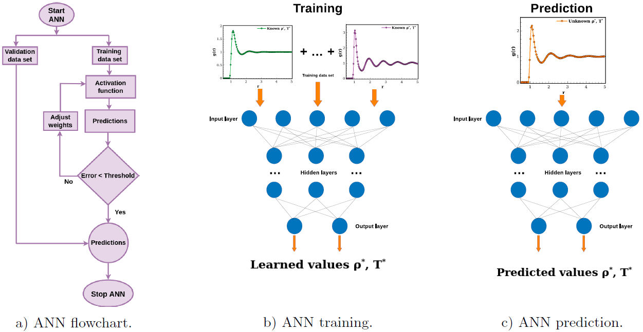
Figure 1 a) Flowchart of the ANN training. Pictorial representations of the b) training and c) prediction stages of the ANN.
In this context, the feed-forward ANN is the most commonly architecture employed and this consists of a number of neurons within interconnecting layers which are distributed as [30]: one input layer, hidden layer(s) and one output layer. In practice, the implementation of an ANN consist of two main stages, namely, i) training (Fig. 1b) and ii) predictions (Fig. 1c), where in each one an independent data-set must be used. Such data are established as is discussed further below.
Thus, using the Python language we implement from scratch a feed-forward ANN whose architecture consists of the input layer with 101 neurons, four hidden layers with 404, 202, 101 and 10 neurons, respectively, and the output layer with two neurons that performs the density and temperature predictions. The Adam optimization algorithm [31] with a learning rate γ = 0.001 [32] along with the rectified linear unit [33] (ReLU) as an activation function were used in order to minimise the error between the real function and the predicted one during the learning stage.
The assessment of the training stage is mainly determined through the mean absolute error (MAE) and the mean squared error (MSE) whose obtained values were 7.7 ×10⁻³ and 1.4 ×10⁻⁴ respectively. Nevertheless, the accuracy of the prediction stage is evaluated individually instead to perform a statistical analysis. This procedure allows us to clearly identify the prediction performance of the ANN at specific thermodynamic regions since we can determine in the magnitude of deviations and identify systematic errors. Then, the ANN prediction accuracy is taken into account through the magnitude of the percentage relative error, defined as 100×(X - XANN)/X, where X stands for the real value of ρ* or T*, respectively. Therefore, XANN is the respective prediction performed by the ANN. This error definition allows us to identify if any individual prediction is underestimated or overestimated through the sign of each result, being positive in the former scenario and negative in the last one.
2.2 Molecular model of simple liquids and training data set
The liquids of interest in this work are commonly referred as noble gases and have been widely studied by experimental, theoretical and computer simulations means. In the last two instances, the interaction between molecules has been modelled by the Lennard-Jones (LJ) fluid with great success. Therefore, we focus on the LJ fluid to make a database to train the ANN. The database is composed of several g(r) determined at different thermodynamic states that spans a wide region in the phase diagram [34].
In particular, we determine the g(r) of the LJ fluid with an analytical equation provided by Morsali et al. [35]. This approach was developed to be accurate in the density and temperature range of 0.35 ≤ ρ* ≤ 1.1 and 0.35 ≤ T* ≤ 4.5, respectively, where
3 Equations of state of molecular liquids
3.1 Prediction of thermodynamic state variables
In this work the accuracy of the ANN is assess performing predictions along thermodynamic states in the isotherms T* = 1.5, 2.5, 3.5 and 4.5.For all fluids studied here these temperatures belong to supercritical states, this election attends to the lack of experimental results at lower temperatures and densities. Thus, once that the ANN is trained we give them a g(r), one that was not used during the learning or validation stages. The ANN predicts the density and temperature at which these g(r) was determined. Results about the prediction accuracy of both density and temperature are shown in Fig. 2. In panel a) density predictions are shown, while temperature predictions are presented in panel b). In the graphs, the error magnitude is associated to a specific colour tone indicated by the bar at the right in each case.
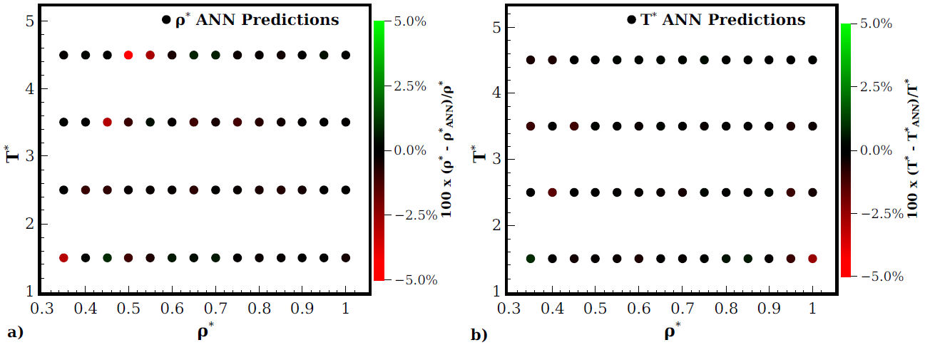
Figure 2 Accuracy of the simultaneous ANN predictions of density and temperature for different thermodynamic states. The error magnitude is shown through the colour map in the bar at the right of each graph. Panel a) and b) shows density and temperature predictions, respectively.
From Fig. 2 it is clear that most of the predictions have a very good agreement, in fact, deviations are lesser than |1%| for both thermodynamic variables. However, there are three states where the density prediction is overestimated, each one belongs to the T* = 1.5, 3.5 and T* = 4.5 isotherms. Nevertheless, although the maximum deviation is around the -5% the prediction can be considered good enough. In fact, considering that only structural information where required, the prediction accuracy is very high. In this sense, one can expect the same degree of accuracy if experimental, theoretical or simulation microscopic structure for similar fluids than the studied here will be used. Furthermore, the ANN architecture could be re-trained to predict the same thermodynamic variables for more complex liquids whose microscopic structure is known in a wide region. Such a task only depends on the quantity and quality of data associated with the microscopic structure available and, in the last instance, on a reasonable assumption of the particular interaction between molecules of such complex liquid.
3.2 Equations of state from ANN predictions
For a thermodynamic description of liquids with theoretical or simulation frameworks usually different equations of state are computed [13], in particular, those that involves the interaction potential and the microscopic structure are the most simplest ones, e.g., the pressure equation of state, given by Eq. (1) or the internal energy equation of state given by
where E/N is the total internal energy per mol. As one can clearly observe from Eqs. (1) and (2) if the microscopic structure g(r) for a given interaction between molecules u(r) is already known, the pressure and internal energy can be determined. Nevertheless, if any, the temperature or density are unknown, such equations are useless.
As we already shown, these thermodynamic state variables can be determined with a high degree of accuracy using our ANN implementation, which, assuming u(r), only needs the information provided by g(r). Thus, encouraged by the good results discussed in Fig. 1, we determined the pressure and internal energy equations of state for different liquids and compared them with the respective experimental results. In order to express the reduced units of density and temperature into real ones we use the respective molecular diameter and energy interaction of the liquid of interest. For the liquids studied here, these parameters can be found elsewhere [36-38].
In Figs. 2 and 4 results for pressure and internal energy of Ar are displayed as a function of density for isotherms at T(K) = 175; 292; 409 and 526. As one can notice, both equations of state are in general well predicted by the ANN, nevertheless, as the density and temperature increases the ANN tends to overestimates the pressure, see for example the isotherm T = 526K in Fig. 3. This behaviour can be traced to the slight overestimation of density predictions at high temperatures, see Fig. 2a).
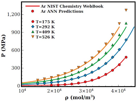
Figure 3 Pressure equation of state as a function of the density for Ar at different temperatures. Lines are experimental available results provided by the NIST data-bank [12] and symbols are results computed with Eq. (1) using the ANN predictions for temperature and density.
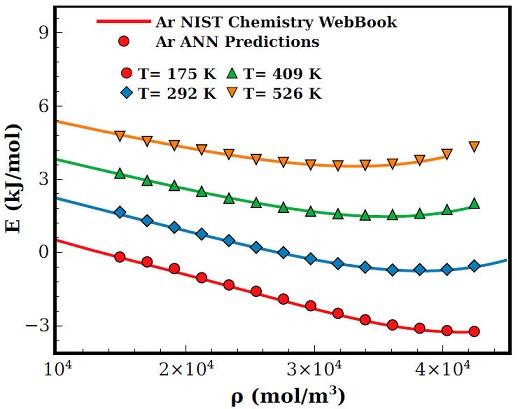
Figure 4 Ar internal energy as a function of the density for different isotherms. Lines are experimental results [12] and symbols are results of Eq. (2) computed with the ANN predictions of density and temperature.
On the other hand, the internal energy prediction within the ANN is remarkably good at any of the studied temperatures as can be seen in Fig. 4.
Although the microscopic structure used to train and predict values with our ANN implementation is well known to be good in the computation of thermophysical properties of Ar [39-41], it should be stressed that a poor estimation of density and/or temperature from the ANN can not give us the good agreement found with the experimental results. At this instance, even the deviations found in the density prediction seems negligible in the computation of the equations of state.
Being that thermodynamic state variables predictions by the ANN have a such good agreement we also compute the pressure and internal energy equations of state for other noble gases, namely, Ne, Kr, and Xe. For these fluids we found that in general the pressure determination is more accurate than the internal energy computation. Actually, for the last property, we observe deviations at high temperatures despite the fluid nature, nevertheless, this behaviour might be an effect of the molecular parameters used to characterise the respective fluid [36-38], however, an improvement of such parameters are out of the scope of this contribution. A comparison between pressure results determined with the state variables predicted by the ANN and experimental ones as a function of density and temperature is shown in Fig. 5. Again, experimental results were obtained from the NIST data bank [12].
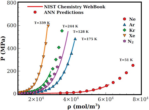
Figure 5 Pressure equation of state as a function of the density for different liquids (Ne, Ar, Kr, and Xe). Lines are experimental results [12] and symbols are the computation of Eq. (1) using the corresponding ANN predictions.
As one can see from Fig. 5, predictions shows a good overall agreement. However, for Kr, as the density is increased we can see an underestimation of the pressure. Nevertheless, such deviations can be due to the molecular parameters (σ and ϵ) used to represent Kr instead to the ANN predictions. Additionally and unfortunately we do not have experimental results at higher densities for Kr. In this regard, a better estimation of those molecular parameters could improve the ANN predictions, however, such task is out of the scope of this contribution. In any case, it is worth to stress the fact that even for densities where experimental pressure results are not reported, the predicted values by the ANN are sound physically meaningful. It means that the ANN could be used to predict such experimental values.
The prediction capabilities of the ANN are also tested against experimental results of some molecular liquids, like N2, CO2, CH4 and C2H4. In Fig. 6a) the pressure behaviour as a function of the density of CH4 for three isotherms is shown. As one can see the agreement is remarkably good, despite that at the highest densities and temperature certain deviations can be seen. Additionally, in Fig. 6b) results for different molecular liquids are also shown, in this scenario CO2 and CH4 are very well predicted but N2 and C2H4 are slightly overestimated, nevertheless, we remark the fact that the qualitative behaviour is well represented.
4 Concluding remarks
Supported by the previously discussed results, we can assure that a straightforward application of ANN algorithms can be safely used to predict thermodynamic state variables in particular situations where only the g(r) is known. Here, we have explored the special case of liquids described by the LJ interaction potential and, using an ANN, supercritical thermodynamic state variables such as density and temperature were predicted. Lastly, such values were used to determine equations of state in the aforementioned regime that also were compared to experimental available results, showing excellent quantitative agreement.
Since the ANN architecture was built and optimised to deal with data related to microscopic structure of liquids, it can be used along other related experimental databases, for instance, that includes thermodynamic states in low density and temperature regime. Another exciting possibility consists in the training of the ANN to predict thermodynamic state variables of different kinds of fluids, like the ones that are commonly used to model colloidal systems, e.g., hard-spheres, square-well or attractive Yukawa fluids among others. Here, the determination of the structure is almost inexpensive but at the same time a correct determination of state variables is fundamental for a complete description considering that data banks of such kinds of systems are scarce.
Nevertheless, it is worth to stress out the paramount relevance of the database used to train any ANN, here, it directly depends on the quality of the microscopic structure data. This impacts the predictions done by the ANN that could be qualitative or quantitative. However, the improvement of the database like the one used in this work can be done by experimental, simulation or theoretical means while the ANN architecture could remain the same and results with the same degree of accuracy can be expected. Work in this direction is in progress.


 nueva página del texto (beta)


