Introduction

The Gulf of California is one of the world's most productive marine ecosystems. It is an eutrophic system with an integrated phytoplankton production (PP) of >1 g C m^-2 day^-1 and in some places >4 g C m^-2 day^-1 (^{Álvarez-Borrego and Lara-Lara 1991}). Average PP for the whole gulf is ~300 g C m^-2 year^-1 (^{Escalante et al. 2013}). Considering the shallow isograms of 45 µmol L^-1 dissolved oxygen, 2.5 µM phosphate (PO₄), and 20 µM nitrate (NO₃), with depths ranging from 50 m to little more than 100 m in the northern Gulf of California (NGC), the gulf's upwelling areas must be among the most productive. These nutrient-rich waters reach the euphotic zone by means of dynamic processes, mainly upwelling and mixing by tidal currents and winds. Surface nutrient concentrations in the NGC may be as high as 1.0 µM PO₄, 4.0 µM NO₃, and 18 µM H₄SiO₄ (^{Álvarez-Borrego et al. 1978}).

The main natural fertilization mechanisms of the Gulf of California are water exchange with the Pacific, upwelling along the eastern coast, and mixing by tidal currents. Other phenomena, such as mesoscale meanders and eddies, also input nutrients to the euphotic zone, but their effect is more local. The net input of NO₃ from the Pacific into the gulf has been estimated at 117 x 10⁹ mol yr^-1 on average, and it is transported to the euphotic zone by upwelling, tidal mixing, etc. This input is much greater than the nutrient input by rivers, which is almost null because of the construction of dams and it has only very local effects (^{Álvarez-Borrego and Giles-Guzmán 2012}).

Seasonality in the Gulf of California is well defined. There are two seasons: "winter", with northwesterly winds, from December through May; and "summer", with southeast erly winds, from July through October, with June and November as transition months. This seasonal cycle has a strong effect on the phytoplankton biomass and PP (^{Hidalgo- González and Álvarez-Borrego 2004}, ^{Kahru et al. 2004}). This is mainly because of the effect of winter upwelling on phytoplankton communities, which is much greater than that of summer upwelling. Surface chlorophyll concentrations (Chl) greater than 10 mg m^-3 have been reported for some eastern regions of the gulf, and because of mesoscale eddy circulation these high concentrations are found across the gulf (^{Santamaría-del-Ángel et al. 1994a}). On the other hand, summer upwelling off the peninsula has a weak impact because of the strong stratification caused by high surface temperatures, resulting in a small Chl increment (up to ~0.5 mg m^-3) (^{Santamaría-del-Ángel et al. 1999}), and because surface flow direction is opposite that of the wind (^{Lluch-Cota 2000}).

The NGC is the shallowest gulf region, with an average depth of ~200 m. It is one of the regions with highest PP, with Chl concentrations of up to 40 mg m^-3, estimated from in situ sampling, and >10 mg m^-3, estimated from satellite data (^{Gendrop-Funes et al. 1978}, ^{Santamaría-del-Ángel et al. 1994a}). In situ PP data (point estimates, with ¹⁴C incubations) for the NGC are scarce, but some values are as high as 2.3gC m^-2 day^-1 (^{Álvarez-Borrego and Lara-Lara 1991}). ^{Hidalgo-González and Álvarez-Borrego (2004)} used satellite data to estimate average PP values for the whole NGC of 61 g C m^-2 day^-1 for winter and of 0.43 g C m^-2 day^-1 for summer. The NGC serves as a reproduction and nursery ground for many invertebrate species, marine mammals, and birds. Its high PP sustains a rich biodiversity consisting of 544 vertebrate and 2258 invertebrate species, of which ~147 are endemic; all together, they represent 47% of the diversity of the entire Gulf of California (^{Brusca et al. 2005}).

Sea bass, sardine, and several shrimp species are the main fishery resources of the NGC. The shrimp trawl fishery is one of the most profitable (^{Cisneros-Mata 2010}); however, this fishery has been responsible for the overharvesting of several species because the shrimp bycatch is ~10 t for each ton of captured shrimp. This bycatch is mainly composed of juveniles of several species. The shrimp fishery has decreased the biodiversity of benthic communities and it has modified the substrate (^{Carvajal et al. 2010}).

The Biosphere Reserve of the Upper Gulf of California and Colorado River Delta was established by federal decree in 1993. Its original purpose was to protect the vaquita (Phocoena sinus ) but a large fraction of its habitat falls outside the reserve. This species is in critical danger. The vaquita's distribution is restricted to 4000 km² in the northwestern NGC (around 30°45'N, 114°20'W) (^{Rojas-Bracho et al. 2006}). A refuge area for the vaquita of 1263 km² was decreed in 2005, but it was extended to 11,000 km² in April 2015.

Over the past three decades controversy has arisen between the fisheries and conservation sectors regarding the management and conservation of the vaquita, because of the ecological problems generated by the fishing activities in this region (^{Brusca et al. 2005}). The hypothesis of the fisheries sector is that the vaquita population has decreased because the lack of freshwater from the Colorado River has negatively impacted the NGC's ecosystem. This hypothesis establishes that with no freshwater there is no nutrient input into the NGC and PP has decreased (^{Galindo-Bect et al. 2000}), causing the pelagic ecosystem to collapse. Yet, there is no proof that nutrient concentrations have diminished significantly, there are no data showing that PP has decreased, and apparently the low nutrient input is not a risk factor for the vaquita in the short term. On the other hand, it has been documented that the vaquita population decline is mainly caused by fishing activities (^{Rojas-Bracho and Taylor 1999}).

The objective of this contribution is to show that the vaquita habitat, and the whole NGC, is a healthy ecosystem in relation to its primary producers (Chl >1 mg m^-3) and that there is no collapse of the pelagic ecosystem because of the lack of nutrients previously supplied by the Colorado River. Several contributions based on satellite data have described the spatial and temporal variation in phytoplankton biomass and PP of the Gulf of California (^{Hidalgo-González and Álvarez-Borrego 2004}, ^{Herrera-Cervantes et al. 2010}, and others cited therein); however, there are no studies describing the details of the large-scale spatial and temporal variation in phytoplankton biomass and PP (synoptic studies) for the NGC. In this contribution we aim to answer the following question: Based on the phytoplankton biomass and PP, is the pelagic ecosystem of the NGC healthy enough to sustain populations of marine mammals such as the vaquita?

Materials and methods

Satellite data

The satellite-derived Chl a (Chl_sat) is the Chl_(z) averaged for the first optical depth (the upper 22% of the euphotic zone), weighted by the irradiance attenuated twice (when the light is going down and when it is back-scattered up) (^{Kirk 1994}). Monthly composites of day sea surface temperature (SST) and Chl_sat were obtained from the NASA website (http://oceancolor.gsfc.nasa.gov/) (level 3 standard mapped image products, 9 x 9 km² pixel size). PP monthly composites were retrieved as a standard product from the Oregon State University (OSU) Ocean Productivity site (http:// www.science.oregonstate.edu/ocean.productivity/index.php). This website provides PP already calculated with the original ^{Behrenfeld and Falkowsky (1997)} vertically generalized production model (VGPM). The VGPM is a non-spectral, homogeneous-biomass vertical distribution, vertically integrated production model.

Data from the CZCS, SeaWiFS, and Aqua-MODIS sensors were used. Chl_sat data were retrieved from all three sensors, but SST and PP were only derived from aqua-MODIS. Satellite imagery was processed with software provided by NASA (SeaWIFS Data Analysis System, SeaDAS 7.0.2) (http://oceancolor.gsfc.nasa.gov/seadas/). To study possible spatial differences of water properties (SST, Chl_sat, and PP), four quadrants were chosen, two in the western (NW and SW) and two in the eastern (NE and SE) parts of the NGC. Each quadrant covered 2025 km² (5 pixels of 9 x 9 km² on each side; a total of 25 pixels). The NW quadrant coincides approximately with the vaquita habitat. Also, a quadrant at Guaymas Basin was chosen, where there should be no effect of the lack of river water and nutrient input, to compare the temporal behavior of Chl_sat data from the three sensors (Fig. 1).

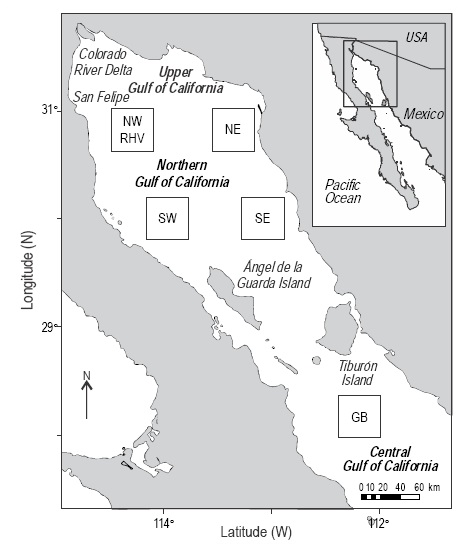
Figure 1 Study area. Location of the four quadrants in the northern Gulf of California and of the Guaymas Basin (GB) quadrant. RHV, vaquita habitat range. 

Time series of SST, Chl_sat, and PP were generated for each quadrant (averages of 25 values per quadrant, per monthly composite). The study period for SST was July 2002 to June 2013, with Aqua-MODIS data. Three time series were generated for Chl_sat: November 1978 to June 1986, with CZCS data; September 1997 to December 2010, with SeaWiFS data; and July 2002 to June 2013, with Aqua-MODIS data. The study period for PP was July 2002 to June 2013, with Aqua-MODIS data. The spectral analysis of time series was performed using ^{Welch's (1967)} periodograms method . To apply this method, low frequencies (interannual variations) were eliminated to filter long-term variation tendencies. As a first approximation to the climatology, an "average yeaf' was generated for each variable and for each quadrant. In the case of Chl_sat, this was also done for each sensor. To do this, data from all Januaries were taken to obtain the "average January" for each variable and for each quadrant, and so on for all months. To generate a true climatology, data from at least 30 years are needed.

Models to estimate phytoplankton productivity

^{Kahru et al. (2009)} and ^{Álvarez-Molina et al. (2013)} reported that the PP values from OSU's Ocean Productivity page (PP_OSU) calculated with the VGPM are overestimated by as much as 50%. To corroborate this, 40 Aqua-MODIS Chl_sat data were chosen at random (10 from each quadrant), and independent PP estimates were performed to compare them with PP_OSU. ^{Platt et al.'s (1991)} model, as modified by ^{Hidalgo-González and Álvarez-Borrego (2004)}, was used to calculate these independent PP values. ^{Platt et al.'s (1991)} model considers a non-homogeneous Chl vertical distribution that takes into account the deep Chl maximum. ^{Hidalgo- González and Álvarez-Borrego (2004)} applied this model to case I waters (Chl <1.5 mg m^-3) and case II waters (Chl > 1.5 mg m^-3). For case II waters, ^{Platt et al.'s (1991)} original model was used. This is a non-spectral model that estimates PP without taking into consideration the change of light quality with depth (eq. 1):

where P* _m is the maximum photosynthetic rate at optimum light, normalized per unit Chl, in mg C mg Chl^-1 h^-1; α*_PAR(z) is the initial slope of the photosynthesis-irradiance relationship (P-E curve), in mg C mg Chl^-1 h^-1 (µmol quanta m^-2 s^-1)-1; and PAR is the photosynthetically active radiation, in µmol quanta m^-2 s^-1. Integration of equation 1 with depth provides PP_PS. For case I waters, the model was modified with ^{Giles-Guzman and Alvarez-Borrego's (2000)} expression for the chlorophyll-specific absorption coefficient of phytoplankton (ā* _ph( _{z Chl} )). This modification corrects the initial slope of the photosynthesis-irradiance relationship for the spectral distribution of in situ scalar PAR and for the package effect. The expression 43.2 Ф _max ^a*p _{h(z Chl)} is used instead of the initial slope α_PAR(z) (eq. 2). The factor 43.2 converts mol C to mg C, seconds to hours, and mol quanta to µmol quanta; Фmax is the maximum photosynthetic quantum yield at low irradiance in mol C (mol quanta)^-1; and a* _{ph (z Chl)} is the weighted average of the specific absorption coefficient of phytoplankton, in m² (mg Chl)^-1, where the weighting factor is the shape of the spectral distribution of in situ PAR (^{Giles- Guzman and Alvarez-Borrego 2000}):

Integration of equation 2 with depth provides PP_GGAB. Equations 1 and 2 show that, to calculate PP, vertical profiles of Chl(_z) and PAR are needed, not only the surface values (^{Hidalgo-Gonzalez and Alvarez-Borrego 2004}). The Chl(_z) vertical profiles were generated from Chl_sat and the Gaussian model proposed by ^{Platt et al. (1991)}, using the parameters reported by ^{Hidalgo-Gonzalez and Alvarez-Borrego (2001)} for the NGC (their winter region IV and summer region 2). Monthly Aqua-MODIS composites for PAR incident on the sea surface (PAR₀) were used. This PAR₀ is the integral for the whole day (daylight hours), also called diurnal insolation Q, and it is expressed as Einstein m^-2 day^-1 (one Einstein is one mole photons, it is Avogadro's number of photons = 6.022 x 10²³ quanta). These values were transformed to µmol quanta m^-2 day^-1. PAR for noon is PAR_m = Qπ/2N, where N is the daylight in seconds. PAR incident on the surface for each hour is PAR(t) = PAR_m sin(πt/N), where t is time in seconds from sunrise (^{Kirk 1994}). PAR(_z) profiles for case I waters were generated following ^{Giles-Guzman and Alvarez- Borrego (2000)}, and for case II waters they were generated following ^{Cervantes-Duarte et al. (2000)}. ^{Valdez-Holguin et al.'s (1999)} values for the photosynthetic parameters (P*m _{z) , αPAR(Z) , and Ф _max) were used. PP was calculated for each morning hour and multiplied by two to obtain PP for the whole day (symmetry of PAR and constancy of Chl_w were assumed for the day).

Results

The SST values for the NGC presented a very clear annual oscillation (15-31 °C). The time series for the four quadrants showed very similar SST values. SST minima occurred in February and March, and maxima in August and September (Fig. 2a). The differences between the summer and winter SST values were significant (Mann-Whitney U test: n = 436, z = -17.72, P < 0.001). The highest winter mean SST was 19.98 ± 0.75 °C (in this and all following cases the number after ± is the standard error, s/n⁰⁵⁾ in the SW quad rant in 2002-2003; the differences with the winter mean SST values for the other quadrants were smaller than the standard error. The winter of 2010-2011 had the lowest mean SST, with 18.4 ± 0.86 °C in the SE quadrant. On the other hand, .the lowest summer mean SST was 28.87 ± 0.78 °C in the NE quadrant in 2002, whereas the summer of 2012 was the warmest, with 30.75 ± 0.76 °C in the NW quadrant. However, SST did not present a significant interannual variation. Winter SST values showed no significant differences between years (Kruskal-Wallis test: n = 260, H = 13.41, P = 0.20), and neither did the summer SST values (Kruskal-Wallis test: n = 176, H = 14.09, P = 0.16). The spectral analysis showed that the seasonal cycle explained most of the SST variability in all four quadrants. This signal was the only significant one (Fig. 2b). The four spectra are very similar, and show a very small, but not significant maximum in the semiannual cycle.

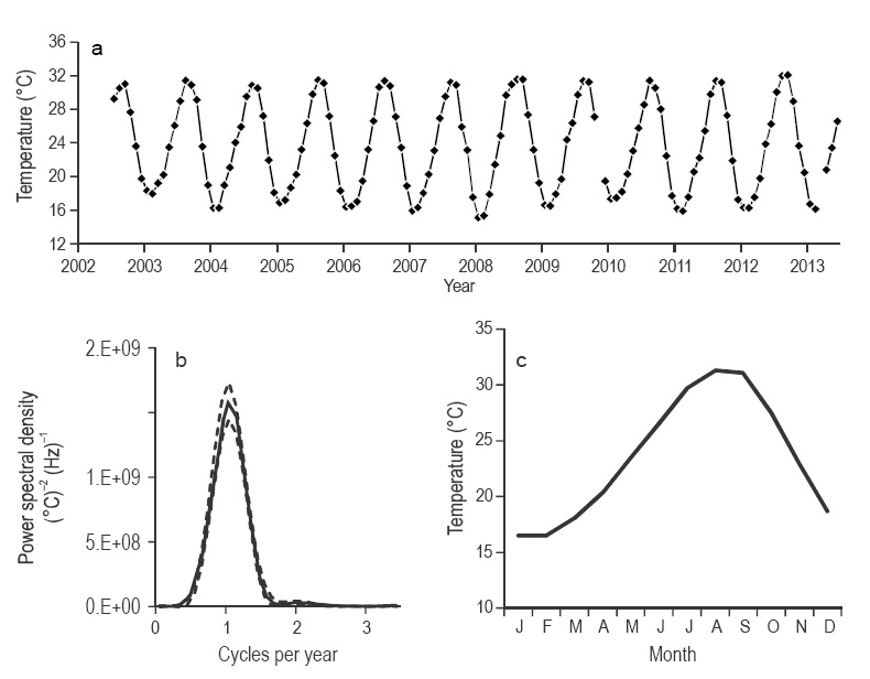
Figure 2 Sea surface temperature (°C). (a) Time series of data from the NW quadrant: the standard error is smaller than the symbols and the marks on the horizontal axis indicate the beginning of the year. (b) Spectral density of data from the NW quadrant: the continuous line is the average and the broken line marks the limits at the 95% confidence level. (c) Average year for the NW quadrant. 

In relation to the approximation to the climatology, the mean SST for February was the lowest, with 16.51 ± 0.23 °C in the NW quadrant, and the mean for August was the high est, with 31.31 ± 0.12 °C also in the NW quadrant (Fig. 2c). There were no significant differences between quadrants in both seasons (Kruskal-Wallis test: n = 260, H = 0.56, P = 0.90 for winter; and n = 176, H = 5.74, P = 0.12 for summer).

The time series from the three sensors show a clear difference between winter and summer Chl_sat values in the NGC (Figs. 3, ⁴ ). Chl_sat showed components of seasonal and between-year variation during the 1978-1986 period (CZCS). The CZCS composites, unlike the imagery from the other sensors, often lacked data for the NW quadrant (Figs. 3, ⁴ ). In general, the NW quadrant had the highest mean Chl_sat values and the SE quadrant the lowest. The CZCS time series for the four quadrants showed a very clear seasonal variation (0.4 to 5 mg m^-3), with minimum values in summer and maximum in winter. There were significant differences between the summer and winter Chl_sat values (Mann-Whitney U test: n = 256, z = 9.83, P < 0.001). Besides the seasonal and interannual variations, Chl_sat had a semiannual variation that can be seen as a secondary maximum in the time series for the four quadrants. This other maximum was much smaller than the one for winter and was (CZCS). A diferencia de las imágenes de los otros sensores, las del CZCS tuvieron muchos vacíos en el cuadrante NW (Fig. 3, ⁴ ). En general, el cuadrante NW presentó los valores promedio de Chl_sat más altos y el SE los más bajos. Las series de tiempo del CZCS de los cuatro cuadrantes presentaron una observed more clearly in the NW quadrant than in the others. It occurred in different times of different years, between the end of summer and end of autumn, and sometimes instead of a peak it was a shoulder (Figs. 3, ⁴ ).

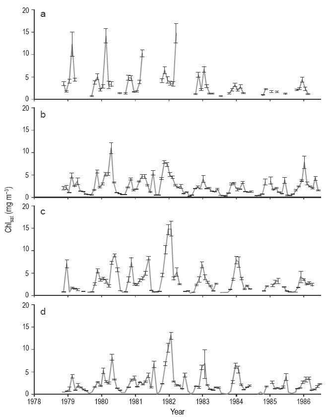
Figure 3 Time series of CZCS Chl_sat data for the four quadrants, for the period 1978-1986: (a) NW, (b) NE, (c) SW, and (d) SE. Vertical bars show the standard error. Marks on the horizontal axis indicate the beginning of the year. 

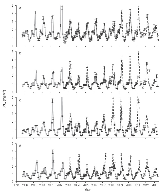
Figure 4 Time series of Chl_sat data from SeaWiFS (continuous line) and Aqua-MODIS (broken line) for the four quadrants, for the 1997-2013 period: (a) NW, (b) NE, (c) SW, and (d) SE. Vertical bars show the standard error. Marks on the horizontal axis indicate the beginning of the year. 

The internannual differences between the CZCS Chl_sat values for the winter months were significant (Kruskal-Wallis test: n = 167, H = 31.66, P < 0.001). The winter of 1981-1982 had the highest mean Chl_sat, with 8.46 ± 2.95 mg m^-3 in the NE quadrant, although differences between quadrants were smaller than the standard error. The winter of 1984-1985 had the lowest, with 1.7 ± 0.04 mg m^-3 in the NW quadrant, again without significant differences between quadrants. On the other hand, the internannual differences between the CZCS Chl_sat values for the summer months were not significant (Kruskal-Wallis test: n = 89, H = 12.88, P >0.05).

The SeaWiFS and Aqua-MODIS Chl_sat time series behaved very similar to the CZCS time series, with semiannual, annual, and interannual variations; however, when both sensors overlapped, the Aqua-MODIS winter Chl_sat values were higher than those from SeaWiFS, while the summer Chl_sat values from both sensors were similar (Fig. 4). Linear regression analysis was performed for SeaWiFS vs Aqua- MODIS Chl_sat with data from the period when both sensors operated at the same time, in order to decide on whether it was appropriate to use both data sets as a single time series. The regression had a slope of 0.73 ± 0.014 and r ² = 0.88 using all data. Separating the data into case I waters (Chl_sat <1.5 mg m^-3) and case II waters (Chl_sat > 1.5 mg m^-3), the regression for case I waters had a slope of 0.86 ± 0.017 and r² = 0.9, while that for case II waters had a slope of 0.21 ± 0.66 and r² = 0.11. In general, in both cases, the Aqua- MODIS Chl_sat data were higher than the SeaWiFS data, but they were very similar in the case of small Chl_sat values, whereas in the case of large Chl_sat values, the Aqua-MODIS data were higher and more scattered than the SeaWiFS data. Thus, both sets of data must be treated separately.

Comparing the SeaWiFS Chl_sat values for the winter months, the interannual variation was significant (Kruskal-Wallis test: n = 300, H = 23.28, P = 0.02). The lowest mean SeaWiFS Chl_sat was 0.76 ± 0.06 mg m^-3 in the SE quadrant in 1997-1998. The interannual variation of the SeaWiFS Chl_sat values for the summer months was not significant (Kruskal-Wallis test: n = 205, H = 13.35, P = 0.42). Aqua-MODIS Chl_sat values for the winter months did not show a significant interannual variation (Kruskal-Wallis test: n = 264, H = 12.80, P = 0.23), with the same result for the interannual variation of the summer months (n = 176, H =9.26, P = 0.50).

The NW quadrant Chl_sat values were higher than those of the other three quadrants throughout the time series from the three sensors (for CZCS data, Kruskal-Wallis test: n = 89, H = 14.5, P = 0.0023; and similar for data from the other sensors). The lowest Chl_sat values were very similar in the other three quadrants. The difference between the NW quadrant and the other three is made clearer by the summer data. During the CZCS period, the lowest summer value for the NW quadrant was >1 mg m^-3, whereas it was ~0.4 mg m^-3 for the other quadrants. During the SeaWiFS and Aqua-MODIS periods, minimum summer Chl_sat values were >0.9 mg m^-3 for the NW quadrant, and they were 0.3-0.4 mg m^-3 in the other quadrants. This Chl_sat spatial variation was not clear for winter. Winter Chl_sat data from CZCS and Aqua-MODIS showed no significant differences between quadrants (Kruskal-Wallis test: n = 167, H = 2.46, P = 0.46; and n = 264, H = 6.4, P = 0.93, respectively), while those from SeaWiFS showed significant differences, with values for the NW quadrant higher than those for the other quadrants (Kruskal-Wallis test: n = 300, H = 54.03, P <0.001).

The approximation to the Chl_sat climatology in the NGC shows a very clear seasonal variation for the three sensors (Fig. 5a-b). The highest mean Chl_sat values are those of March and April in the case of SeaWIFS and Aqua-MODIS, and those of February, November, and December in the case of CZCS. In all three cases, there are two maxima, but they were clearer in the CZCS climatology. Winter CZCS values were more than double those of the other two sensors. The lowest mean Chl_sat values were observed in July, August, and September, and they were very similar for the three sensors. As a comparison, the climatology for Guaymas Basin also shows that the winter CZCS values are more than double those of the other sensors (Fig. 5c).

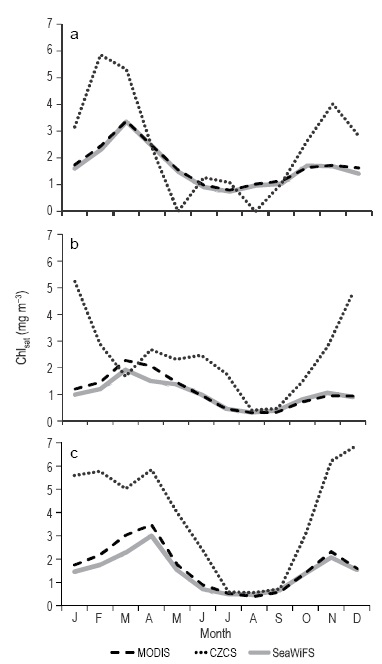
Figure 5 Approximation to the Chl_sat climatology of the (a) NW and (b) SE quadrants in the northern Gulf of California and (c) Guaymas Basin quadrant. The broken line represents Aqua- MODIS data, the dotted line represents CZCS data, and the continuous line represents SeaWiFS data. 

Linear regression analysis to explore the possibility of a long-period Chl_sat trend, run separately for each sensor and for each quadrant, resulted in low correlation coefficients and non-significant slopes (for the NW quadrant and for data from the three sensors: n = 31, F = 2.73, P = 0.11; n = 96, F = 0.35, P = 0.55; and n = 66, F = 1.10, P = 0.30, respectively for CZCS, SeaWIFS, and Aqua-MODIS). The spectral analysis showed a strong annual signal (seasonal cycle) that causes most of the Chl_sat variability in the NGC. It also showed a Chl_sat semiannual signal (two cycles per year), but smaller than the annual and only significant for data from Aqua- MODIS, at the 95% confidence level (Fig. 6a-b).

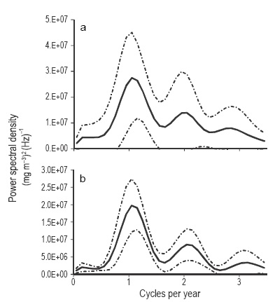
Figure 6 Spectral density of Chl_sat for the NW quadrant: (a) SeaWiFS data and (b) Aqua-MODIS data. The continuous line is the average and the broken line marks the limits at the 95% confidence level. 

The NGC PP showed a spatial and temporal variability very similar to that of Chl_sat, with a clear difference between winter and summer values (2002-2013 period) (Fig. 7a-b). Besides the seasonal variation, PP had a semiannual component, which was corroborated by the spectral analysis (Fig. 7c). The interannual variation was not significant (Kruskal-Wallis test: n = 264, H = 11.67, P = 0.30 for winter; and n = 176, H = 9.27, P = 0.50 for summer). In general, the NW quadrant had the highest average PP, mainly in summer. In the first approximation to the PP climatology, March and April were the most productive, with ~3.3 ± 0.2 g C m^-2 day^-1. On the other hand, the period July-September was the least productive, with ~1.1 g C m^-2 day^-1 in the NW quadrant and 0.5-0.6 g C m^-2 day^-1 in the other quadrants (Fig. 7d).

Figure 7 Primary production. Time series for the (a) NW quadrant and (b) SE quadrant: vertical bars show the standard error and the marks on the horizontal axis indicate the beginning of the year. (c) Spectral density of data from the NW quadrant: the continuous line is the average and the broken line marks the limits at the 95% confidence level. (d) Average year for the NW quadrant. 

Of the 40 Chl_sat and PAR data chosen at random to calculate PP using ^{Platt et al.'s (1991)} model, 28 were for case I waters and 12 were for case II waters. For case I waters, the slope of the PP_OSU vs PP_GGab relationship was 2.817 ± 0.008, thus PP_OSU was up to ~3 times PP_GGab. Linear regression analysis was statistically significant (n = 28, F = 90.53, P <0.001), with a relatively high correlation coefficient (r = 0.79) (Fig. 8a). For case II waters, the slope of the PP_OSU vs PP_PS relationship was 0.446 ± 1.233; thus, in general, PP_OSU was smaller than PP_PS (PP_OSU was greater than PP_PS only in two cases). Linear regression analysis, however, was not statistically significant (n = 12, F = 1.33, P = 0.274) (r = 0.42) (Fig. 8b).

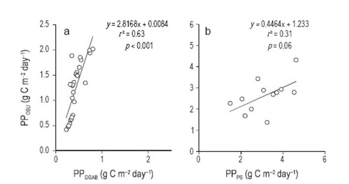
Figure 8 Linear regression between primary productivity (PP) data from Oregon State University's Ocean Productivity website (PP_Osu) and PP estimated with ^{Platt et al.'s (1991)} model for (a) case I waters and (b) case II waters. 

Discussion

The record of the Colorado River flow across the Mexico-Us border shows that before 1935, when the filling of Lake Mead (Hoover Dam) began, the freshwater that was discharged into the Uper Gulf had a seasonal modulation with peak discharges in June. After construction of the Glen Canyon Dam, input of Colorado River water to the Upper Gulf completely stopped (in 1961). During 1979-1987, water releases became necessary because of abnormal high precipitation and snowmelts in the upper river basin. Water releases also occurred in 1993 and 1997-2002 (^{Álvarez-Borrego 2002}). Before the dams, there was a large interannual variation of river flow into the Upper Gulf, with a maximum of >32 x 10⁹ m³ yr^-1 and a minimum of <10 x 10⁹ m³ yr^-1 in the first 30 years of the 20th century. The largest water release in the period 1979-1987 was >15 x 10⁹ m³ yr^-1, similar to that of the river flowing freely.

When the Colorado River flowed freely, its influence was restricted to a few tens of kilometers to the southwest of the mouth, and was not felt throughout the whole NGC. ^{Lavín and Sánchez (1999)} reported that when the river flowed into the sea in 1993, the river plume with significantly mixed water only extended ~70 km southwestwards from the mouth, close to the peninsula. ^{Rodríguez et al. (2001)} used ¹⁸O in shells of a bivalve endemic to the Colorado River estuary (Mulinia coloradoensis Dall 1894) to reconstruct the river influence area before the construction of the dams and concluded that it extended to a maximum of ~80 km to the southwest of the mouth.

^{Nieto-García (1998)} compared nutrient concentrations in the Upper Gulf in the spring of 1993 with those of spring 1996, when there was no water input from the Colorado River, and found that NO₃ and PO₄ concentrations were lower in 1993 than in 1996, and only silicate concentrations were higher in 1993. When comparing our Chl_sat data for wet years with those of dry years, the differences were not signif icant. Thus, processes like mixing caused by tidal currents and coastal upwelling are causing the NGC to be productive, and nutrients from the Colorado River are not necessary to maintain its high PP.

^{Galindo-Bect et al. (2000)} reported that higher shrimp catches landed in San Felipe were associated with river water discharges in the period 1976-1996, and a log-log regression with a one-year lag for the catches explained 45% of the variance. ^{Aragón-Noriega and Calderón-Aguilera (2000)} indicated that an important factor explaining the shrimp population increase is that expanded habitat (wetlands for shrimp larvae, postlarvae, and juveniles) is available when the Colorado River flow increases, because freshwater floods areas that are dry in those years when river discharge is null or too low. Furthermore, a commercial fishery for the Gulf corvina, Cynoscion othonopterus, a fish endemic to the Upper Gulf of California, existed from 1917 to 1940 but collapsed in the early 1960s. This collapse was attributed to fishing practices and the reduction in flow of the Colorado River into the Gulf of California, which supposedly reduced available nursery habitat for juveniles (^{Román-Rodríguez 2000})Nevertheless, the corvina fishery reappeared during the 1990s and continues to date (^{Aragón-Noriega 2014}), in spite of the general lack of freshwater input to the Upper Gulf.

In general, the NGC has been considered a highly productive region. High winter Chl_sat values ranging from 1 to >5 mg m^-3 have been reported (^{Santamaría-del-Ángel etal. 1994a}). Strictly, it is not appropriate to compare Chl_sat and satellite-derived PP data with those from oceanographic cruises, because the two data sets have totally different time and space scales: satellite data are averages for 9 x 9 km² areas and for one month, whereas data from oceanographic cruises are instantaneous point measurements. Nevertheless, the comparison is interesting. Winter Chl data generated during oceanographic cruises also ranged from 2 to >5 mg m^-3, with very few values of up to 20 mg m^-3 (^{Gendrop-Funes et al. 1978}, ^{Álvarez-Borrego and Gaxiola-Castro 1988}, ^{Gaxiola-Castro et al. 1995}, ^{Valdez-Holguín et al. 1995}), similar in general to the Chl_sat data presented in this study. Time series of Chl data generated from in situ sampling at sites close to the coast off San Felipe (Baja California) and Santa Clara (Sonora) show values <1.0 mg m^-3 for September, values between ~1.5 and >5 mg m^-3 for February, and values >20 mg m^-3 for May (^{Álvarez-Borrego 2002}), again similar to the Chl_sat values presented here. ^{Álvarez-Borrego and Lara-Lara (1991)} reported only six ¹⁴C PP data points for the NGC, ranging from 0.6 to 2.3 g C m^-2 day^-1, with the highest values for June and lowest values for November. ^{Álvarez- Borrego and Lara-Lara's (1991)} low values agree with our summer values, but their high winter values are only about 70% of the satellite-derived PP values. Although point and instantaneous ¹⁴C PP data are extremely scarce, the comparison indicates that satellite-derived values might be overestimating PP.

The main source of interannual changes in the ocean climate of the Gulf of California is the El Niño influence (^{Baumgartner and Christensen 1985}), and this also applies to Chl_sat. The 1982-1983 El Niño, which affected the Gulf of California throughout 1984, and the 1997-1998 El Niño occurred during our study period (^{Santamaría-del-Ángel et al. 1994b}, ^{Hidalgo-González and Álvarez-Borrego 2004}), both of the Eastern Pacific type. ^{Santamaría-del-Ángel et al. (1994b)} reported a decrease in Chl_sat values for the winters of 1982-1983 and 1983-1984 relative to the 1981-1982 values, but they reported that the impact was not the same throughout the gulf. In the NGC and the region of the big islands, Chl_sat differences between El Niño years and non-El Niño years were not significant, while differences were very clear for southern localities. Likewise, the effects of the 1997-1998 El Niño on the NGC were less evident than in the southern gulf (^{Hidalgo-González and Álvarez-Borrego 2004}, ^{Kahru et al. 2004}). In this study, a significant decrease in Chl_sat for the winter of 1983-1984 with respect to that for 1981-1982 is reported, due to the effect of El Niño, in spite of the large Colorado River water input of 1984. Also, this study reports a significant decrease in Chlsat values for the winter of 1997-1998 with respect to those for 1999-2000, for the four quadrants, because of the 1997-1998 El Niño, in agreement with the values for the whole NGC reported by Hidalgo- González and Álvarez-Borrego (2004), and Kahru et al. (2004), again in spite of the Colorado River water input. However, the NGC Chlsat values were not lower than 1.0mgm^-3 in the case of both 1982-1984 and 1997-1998. The decrease in Chl_sat in 1997-1998 was similar in the four quadrants of the NGC (Fig. 4), contrary to what ^{Herrera- Cervantes et al. (2010)} reported. These latter authors con cluded that the effect of the 1997-1998 El Niño was greater in the northwestern portion than in the rest of the NGC. Aqua-MODIS Chl_sat did not show any El Niño effect because the events of the 2002-2013 period were of the Central Pacific type.

The semiannual component of variation is caused by the sequence of intense stratification during summer and mixing during autumn due to mesoscale processes, such as the change from cyclonic to anticyclonic circulation as described by ^{Lavín et al. (1997)}. In early autumn, stratification weakens and because of the effect of mixing processes nutrients are transported to the euphotic zone, although not as efficiently as with coastal upwelling, generating a secondary Chl_sat maximum in October (Figs. 3, ⁴ ).

The PP graphs parallel those of Chl_sat (Figs. 4, ⁷ ). Even though the calculated PP fields depend on SST, PAR, and daylength, Chl_sat dominated the variability in PP, as was also reported by ^{Kahru et al. (2004)} and ^{Álvarez-Molina et al. (2013)} for the whole gulf. ^{Hidalgo-González and Álvarez- Borrego (2004)} and ^{Kahru et al. (2004)} reported that the seasonal cycle is the one with most Chl_sat and PP variation in the NGC. Since several decades ago, it is well known that the Chl_sat and PP seasonal cycle is strongly determined by upwelling events caused by northwesterly winds off the continental coast during winter and strong stratification during summer due to southeasterly winds (^{Álvarez-Borrego and Lara-Lara 1991}).

The high Chl_sat values from CZCS were clearly higher than those from SeaWiFS and Aqua-MODIS, which could lead us to conclude that there has been a decrease in phytoplankton biomass from the 1970s and 1980s through the 2000s, because of the deterioration of the NGC's pelagic ecosystem caused by the lack of Colorado River water and its nutrients. However, these Chl_sat differences could have been caused by differences in the optical design of the sensors and not by changes in the environmental conditions of the NGC. For example, ^{Kahru et al. (2012)} reported differences between the Chl_sat values deduced from four sensors (OCTS, SeaWiFS, Aqua-MODIS, and MERIS) for the California Current System. In this study, differences between sensors are proven with Chl_sat data from Guaymas Basin, which is a region with very high winter Chl_sat and PP values, and where there is no effect caused by the lack of nutrients from rivers. High Chl_sat data from CZCS for the Guaymas Basin were also clearly much higher than those from the other two sensors, very similar to that observed for the NGC (Fig. 5c). Thus, CZCS overestimates Chl_sat values higher than 0.5 mg m^-3 by as much as >5 times (Fig. 5).

The summer Chl_sat and PP differences between the NW and the other quadrants were caused by the greater concentrations of organic matter in the former, both as detritus and as color dissolved organic matter (CDOM). These optical components of seawater strongly attenuate light at short wavelengths (^{Kirk 1994}), and the satellite sensors detect the sum of their effects as if they were only caused by Chl, generating higher Chl_sat values. The greater concentrations of detritus and CDOM in the NW quadrant are caused by the summer cyclonic circulation that transports water from the Upper Gulf of California southward, in the northwestern part of the NGC (^{Alvarez-Borrego 2001}). In general, in the Upper Gulf turbidity increases towards the northwest, with Sechii disk depths of 2 m in relatively deep waters and of 0.5-1 m near the Baja California coast. In the most turbid areas, seston values are >130 mg L^-1, with almost 100% of organic particles (^{Garcia-de-Ballesteros and Larroque 1976}).

^{Santamaria-del-Angel et al. (1994a)} reported that throughout the Gulf of California, the Chl_sat maxima occurred off the eastern coast, during winter upwelling events. In the NGC, however, winter Chl_sat maxima for the eastern quadrants showed no significant differences from those for the western quadrants. This could be attributed to the circulation in this region that carries water from one side of the NGC to the other relatively quickly, since it is the narrowest part of the gulf. A water parcel takes ~10 days to travel from one side to the other of the NGC, and phytoplankton biomass does not decrease significantly during the trajectory.

Aknowledgements

MR Ramirez-Leon was granted a postgraduate scholarship by the National Council for Science and Technology (CONACYT, Mexico). FJ Ponce helped with the graphical design. The comments made by two anonymous reviewers helped to improve the manuscript.