1. Introduction

Nowadays, most of the world's population lives in urban areas. According to a United Nations report (^{UN, 2015}), 54% of the current world’s population lives in cities and this proportion is expected to increase to 66% by 2050. Unfortunately, the high concentration of human activities (i.e., heating, transport, nutrition, hygiene, health, and other needs) in urban areas involves emissions from the consumption of fossil fuel energy sources; therefore, large amounts of pollutants are released daily into the urban atmosphere. The impacts of this phenomenon on human health are well known; air pollution triggers stroke, cardiovascular and respiratory diseases, which are featured among the top 10 killers in the world (^{WHO, 2017}).

Latin American cities have also experienced important deterioriation in air quality (^{Bell et al., 2011}; ^{Hanif, 2017}; ^{Román Collado and Morales Carrión, 2018}). According to ^{Gouveia and Leite (2018)}, Mexico City, Santiago de Chile, Sao Paulo, and Rio de Janeiro host nearly 43 million people and have a large child population exposed to levels of air pollution well above those recommended by the World Health Organization (WHO) guidelines. Statistical evaluations showed significant impacts of air pollution on respiratory mortality in children (Gouveia and Leite, 2018), and health risks markedly higher near sources of pollution (^{Brugge et al., 2013}). The pollution stemming from transport has been significant and growing (^{Faiz et al., 1995}).

In Havana, epidemiologic studies pointed out associations of health hazards proportional to ambient PM_2.5, PM₁₀, NO₂ and SO₂. ^{Molina Esquivel et al. (1996)} found increased risk of lung cancer by predominant residence (≥ 40 yrs) in SO₂ and PM₁₀ high polluted areas. ^{Molina Esquivel et al. (2011)} reported high PM₁₀ concentration associated with morbidity and mortality rates. Daily mean black smoke concentration increments of 20μg m^-3 and SO₂ were associated with increments of 2.4% on child acute respiratory infections in the period from October 1996 to March 1998 (^{Romero Placeres et al., 2004}); and correlations between daily mean concentrations, meteorological parameters (i.e., temperature, wind speed, and direction) and respiratory morbidity indicators showed respiratory diseases highly influenced by PM₁₀ values reaching WHO risk limits on the period from October 1996 to September 1997 (^{Molina Esquivel et al. 2001a}, ^b). Most of these studies recurrently point to PM as the pollutant with major impact on the health of Havana citizens and attribute the high levels of PM_2.5 and PM₁₀ pollution to the poor technical condition of vehicles (^{Molina Esquivel et al. 2015}, ²⁰¹⁷).

Designating transport as a likely source of Havana air pollution issues is usually supported by arguments referring to a mainly old vehicle fleet (most models are American from the 1950s or Russian from the 1980s) with low fuel efficiency and high emission systems (cf. ^{Ding et al., 2004}; ^{Romero Placeres et al., 2004}; ^{Molina Esquivel et al., 2001a}, ^b, ²⁰¹¹, ²⁰¹⁷; ^{Martínez Varona et al., 2011}). Only a few studies have relied on the use of tools to report evidence (cf. Molina Esquivel et al., 2015; ^{Martínez Varona et al., 2018}). Their measurements have been obtained from 24-h data collected with passive samplers, then followed by chemical analysis in the laboratory. For PM, low volume gravimetric analytical methods were used, while SO₂ and NO₂ gases were measured by diffusive devices (spectrophotometric, absorption method) with a minimum 24-h sampling exposition. These setting techniques may not reproduce conditions where pollutant concentrations (particles or gases) fluctuate or are inhomogeneous, such as in transport-related pollution. So far, evidencing traffic-related air pollution has been a challenge, since passive monitoring can only detect the concentration of ambient air pollution caused by various factors as a whole (^{Cuesta Santos et al. 2012}; ^{Pan et al. 2016}).

In this work, we explore traffic-generated pollution in Havana by analyzing shorter-time correlations between traffic flows, pollutant concentrations and meteorological parameters. We consider that this approach avoids the difficulty of discriminating between traffic-related air pollution and ambient air pollution. A measurement campaign was carried out on an important street of Havana where traffic volumes, some traffic-related pollutants (i.e., PM₁₀, SO₂, and NO₂) and meteorological parameters were rated with proper temporal resolution. Then, statistical relationships among all variables were analyzed, aiming to show how strong pollutant measurements are influenced by traffic flows during specific meteorological episodes.

2. Measurement campaign

The measurement campaign took place on Simón Bolívar Street (Fig. 1) close to the center of Havana, during 10 days in the summer of 2015. This street is an urban corridor built prior to the beginning of 20th century where important daily commuting movements take place; it is about 12 m wide with an east-west direction. According to the average height of the surrounding buildings (about 15 m) it is classified as an urban canyon (height/width ratio of 1.25).

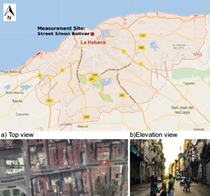
Fig. 1 Location of the masurement site at Simón Bolívar Street in Havana City (red point). Adapted from Google earth map: (a) Street top view with the meteorological station (1) traffic video recording (2), and pollutant measurement devices (3); (b) street elevation view. 

The diurnal traffic flow along the street was continuously recorded with a GoPro video camera placed on the north side of the street, about 200 m away from the nearest traffic light intersection, at a proper elevation to capture all traffic lanes (see Fig. 1 for more details). Traffic volumes were manually counted after the measuring campaign from the video recordings and aggregated into clearly identifiable categories, i.e., motorcycles, modern cars, median-age cars (of Russian origin), old-age cars (of American origin), high-capacity buses, low-capacity buses, and trucks.

Devices for measuring PM₁₀, NO₂, and SO₂ air pollution were installed 1.5 m above the ground. A Thermo-Scientific ADR 1500 was used for PM; it incorporates light scattering photometry, optical sensing and electronic processing techniques to measure precisely a selected size of suspended particles down to 1μg m^-3. It was set to provide real-time PM₁₀ concentrations every minute from 07:00 to 19:00 LT. The concentrations of pollutant gases were captured from chemical adsorption (i.e., a chemical reaction between the given gas and an adsorbing substance). CT-112 and CT-212 bearers (^{Volberg 1982}) of tetrachloromercurate and potassium iodide were used as sorbent tubes sampling for a 1-h step at accurately known flow rates of 1.0 and 0.25 L/min. They were measured by visible spectrophotometric techniques at 540 and 575 nm wavelengths, respectively. The mass of gases in each tube was determined from calibration curves; then concentration levels of SO₂ and NO₂ were calculated by applying the corresponding conversion factors, i.e. 2.830 for SO₂ and 17.294 for NO₂. For both pollutant gases, the limits of detection and quantitation were 0.1 and 500 μg m^-3 respectively. All pollutant measurements were suspended during rainfall episodes to discard events of substantial pollutant concentration decline due to washing out of particles and absorption of pollutants.

A meteorological station and radio wave transmission housing were placed on the roof of the nearest building. This edifice is the highest point (~20 m high) within a 1-km radius. The registered meteorological parameters were temperature, solar radiation, atmospheric pressure, humidity, wind speed, and direction. All data were automatically stored in a computer at a 1-min step resolution.

3. Result and discussion

3.1 Traffic flows

More than 15 000 vehicles were counted daily over the campaign period (Fig. 2). The fleet mainly comprises light-duty cars (i.e., modern cars [27.6%], medium-age cars [16.2%], and old cars [33.0%]). Merely 8.9% of the fleet is comprised by motorcycles and 14.3% by heavy-duty vehicles including buses and trucks. This composition is rather typical in Havana. Figure 2a shows that light-duty categories (especially old vehicles) are responsible for the highest flow variability. In Figure 2b, hourly fluctuations of traffic flow produce wider but visibly distinguishable peaks; during the morning, traffic increases until 11:00 LT and then subtly decreases prior to 17:00 LT, when a new peak appears.

Fig. 2 Traffic data: (a) box plots of vehicle categories, (b) hourly flows. 

3.2 Concentration levels

Hourly diurnal PM₁₀, NO₂, and SO₂ measurements are shown in Figure 3. The PM₁₀ plot was obtained by averaging the 1-min step measurements over 1 h from all data gathered during the campaign. PM₁₀ diurnal average fluctuates close to the mean value ranging from 88 to 115 μg m^-3. NO₂ and SO₂ ranged from 72 to 138 and 14 to 40 μg m^-3, respectively. These values are higher than the means reported on previous studies for PM₁₀ (30-61 μg m^-3), NO₂ (8-20 μg m^-3) and SO₂ (1.5-24 μg m^-3) (^{Molina Esquivel et al., 2001a}; ^{Martínez Varona et al., 2013}; ^{Cruz Rodríguez and Valdivia Pérez, 2017}). These differences could be traced to the use of measurement settings (e.g., sampling height and duration) that differed from the referenced studies.

Fig. 3 Average diurnal variations of PM₁₀, NO₂, and SO₂. 

In Figure 3, the PM₁₀ fluctuations do not seem to follow completely the increase of the middle morning traffic (Fig. 2b); nevertheless, after 11:00 LT a better correspondence with the traffic profile is observed. NO₂ exhibits the highest values on morning hours; before 9:00 LT, the pollutant profile seems to be inversely correlated with traffic flows. However, after noontime, NO₂ levels fall further and then rise around 15:00 LT in a modest accordance with traffic trends. For SO₂, the almost constant temporal profile (with exception of some observations that went beyond limits) suggests that contributions from stable sources are more important than the vehicle ones.

Regarding SO₂ variations, no inferences could be made on whether or not they are interrelated with local traffic flows. Indeed, these pollution trends analyses are indicative of concentration-response at street level from all emission sources; single-handedly, they do not provide conclusive insights about the traffic-generated pollution behavior.

3.3 Meteorological parameters

Meteorological data analysis focused on wind speed and direction as high-influencing parameters of pollutant dispersion. Figure 4 shows wind roses of 3-h intervals (i.e., 7:00-10:00, 10:00-13:00, 13:00-16:00, and 16:00-19:00 LT). Two different regimes can be observed: during the first interval, winds come from the south-southeast at a relatively low speed while on the other periods wind mainly comes from the north-northeast at higher speeds.

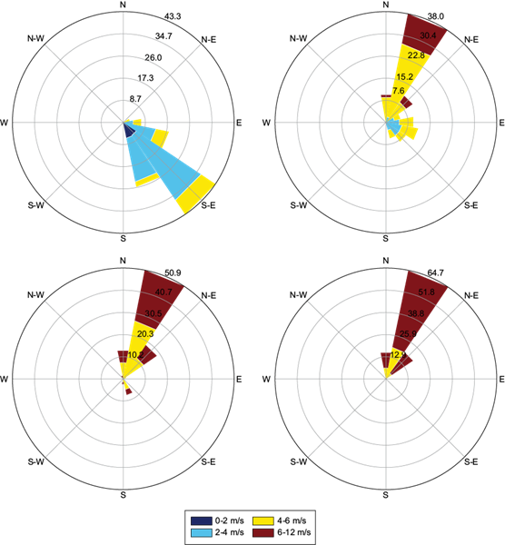
Fig. 4 Wind roses of average diurnal variation of wind forces. 7:00-10:00 LT (top-left), 10:00-13:00 LT (top-right), 16:00-19:00 LT (down-left), and 13:00-16:00 LT (down-right). 

These observations agree with the theory of sea-land breezes suggested by ^{Simpson (1996)}. A delayed offshore breeze can be observed on the first wind rose; on the previous night, the land loses heat quickly after the sun sets down and the air above also cools. Water has much higher thermal inertia (i.e., very little day/night temperature change). The relatively warm air over the sea causes low pressure. Over the land, high surface pressure will develop because of colder air; to compensate, the wind blows from higher pressure over the land to lower pressure over the sea causing a land breeze (^{Ding et al., 2004}). During the middle morning, the wind starts the reverse phenomenon on the so-called sea breeze; the sun heats up both the sea surface and land; however, water heats up much more slowly than land, so the air above land will be warmer compared to the air over the sea. This causes a wind blowing from the sea inland.

It is believed that land-see breezes generate specific pollutant motion regimes inside the street canyon and therefore influence traffic contributions: according to ^{Berkowicz et al. (1997)}, ^{Berkowicz (1998)}, and ^{Kastner-Klein et al. (2003)}, the wind flows at street level and the pollutant recirculation features depend on roof-level wind flows. The street-level wind inside the recirculation zone forms an angle with the street axis, which is equal to that of wind direction at roof level with respect to the street axis but with transverse component (i.e., as a mirror reflection). Outside the recirculation zone, the wind direction is the same that at roof level. Also, the variability of the wind directions across the measurement site may explain the existence of different air pollution behaviors.

3.4 Statistical relationships between traffic flow, pollutant concentration, and wind forces

As aforementioned, the wind flow regimes are expected to influence pollutant concentration levels, since they change the features of pollutant motion and limit the scope of surrounding pollution sources.

In Figure 5, bivariate polar plots allow for understanding the sources of pollution according to prevalent wind flow profiles (i.e., land [7:00-10:00 LT] and sea [13:00-19:00 LT] breezes). During the morning, PM₁₀ tends to be highest (140 μg m^-3) under low and perpendicular (with respect to the street axis) wind conditions, pointing to ground level source contributions such as traffic. NO₂ does not vary with the variation of wind speeds, suggesting also traffic contributions. However, it tends to increase (from 100 to 200 μg m^-3) as wind direction changes from south to east; at this point, contributions from non-traffic sources become more significant with high-speed wind. SO₂ decrease (from 45 to 20 μg m^-3) as wind directions change from south to east and remain almost constant under wind speed fluctuations. This highlights the influence of ground-level sources for wind blowing perpendicularly to the street axis. During the afternoon, pollutants variations were less pronounced compared to the morning. PM₁₀ subtly increases (from 80 to 100 μg m^-3) as wind direction shifts from southeast to northeast. SO₂ tends to peak under high wind speed conditions at northeast, pointing to the existence of important sources other than traffic. NO₂ is less influenced by wind conditions.

Fig. 5 Bivariate polar plot. 

To better emphasize the strength of traffic contributions, statically significant correlations between pollutants and flows of specific vehicle categories, including several alternative aggregation schemes, were set. Best results were found by grouping vehicles of similar emission profiles (i.e., buses and trucks were aggregated on the “Heavy” category, medium and old-age light-duty vehicles were aggregated on the “MedOld” category, and motorcycles and modern light-duty vehicles remained as single categories; see Table I).

Table I Significant correlations (p-value < 0.05)* between pollutants and vehicular flow. 

	Morning 07:00-10:00			Afternoon 13:00-18:00
	PM10	NO2	SO2	PM10	NO2	SO2
Motorcycles	0.68	-	-	0.42	0.49	0.36
	7e-04			6e-03	1e-02	2e-02
Modern vehicles	0.74	-	0.45	0.41	0.47	0.39
	3e-05		4e-02	8e-03	2e-02	1e-02
Med-old vehicles	0.78	-	-	-	-	0.54
	1e-04					4e-02
Heavy	0.63	-	0.53	0.65	0.63	-
	2e-03			1e-02	9e-04	7e-04
Total vehicles	0.83	-	-	0.50	0.53	0.39
	7e-06			1e-02	3e-02	1e-02

*This indicates that there is a 5% risk of concluding that a correlation exists, i.e., changes in vehicle categories are related to changes in pollutant concentration levels.

Morning rises in PM₁₀ are coupled with rises in traffic, indicating that PM₁₀ concentration levels were likely induced by vehicle emissions. The correlation between SO₂ and vehicle emissions is moderate, mostly influenced by heavy vehicles traffic. During afternoons, all pollutants correlate acceptably. PM₁₀ and NO₂ are highly influenced by heavy vehicles, while SO₂ is coupled with changes in old and medium-age vehicles. The statistically significant relationships for variables in Table I indicate that the three pollutants do account for traffic contributions, which increase under specific meteorological conditions.

4. Conclusion

Aiming to evidence traffic-generated air pollution in Havana, statistical tools were applied to a set of pollutant, traffic and meteorological measurements (1-h samples). Statistically significant relationships between hourly traffic and pollutant measurements indicated that PM₁₀, NO₂, and SO₂ account for traffic contributions. Morning PM₁₀ pollution is mostly influenced by traffic. PM₁₀, NO₂ and SO₂ traffic-generated pollution increases with low-speed winds which blow perpendicular to the street axis. In addition to traffic, emissions from other sources seem to be dragged by winds from the southeast/northeast (morning/afternoon) inducing variations, mainly in the pollution levels of NO₂ and SO₂. These conclusions are dependent on specific wind conditions of the Cuban summer season at the measurement area. A more complete analysis could be conducted when more data becomes available for other seasons.