INTRODUCTION
A new coronavirus denominated first 2019-nCoV and later SARS-CoV-2 was found in Wuhan, China in December of 2019 [1] [2] [3] [4] [5]. This new virus has originated a worldwide pandemic [6], worse than the Severe Acute Respiratory Syndrome Coronavirus epidemic (SARS-CoV) and Middle Eastern Respiratory Syndrome Coronavirus (MERS-CoV) epidemic [7] [8] [9]. It is believed that SARS-CoV-2 jump from the bats to humans, the bats were on the markets and restaurants in Southern China with the potential to cause a global outbreak [10]. The World Health Organization (WHO) called it COVID19 disease.
Lin et al. propose in 2020 a conceptual model to control the COVID-19 outbreak. The model includes among other measurements: holiday extension, travel restriction, hospitalization, and quarantine of the population [11]. Additionally, computational advances in the performance of algorithms may help epidemiologists to take decisions in case of outbreaks [12].
Currently, exist mathematical models to predict or simulate an epidemic spread among them: Nonlinear regression [13], SIR [14], SEIR [15]. Other methods exist that use more variables, but they can be used when the pandemic has already produced enough data it means no at the beginning of the pandemic outbreak.
The Nonlineal model has been used to estimate the impact of the COVID-19 from a global perspective in Germany [13].
The effectiveness of modeling the COVID-19 pandemic with the SIR model was evaluated in 6 countries [14]. And the SEIR epidemic model was employed to build some general control strategies [15]. These three models were chosen because they consider variables that can be known during the epidemic beginning, making it possible to calculate the prediction of the infected people in any country.
The SIR model analyses different variables like the number of people susceptible to sickness, S(t), the number of infected persons, I(t), and the removed people free of spread infection or recovered people, R(t) [16] [17].
The SEIR model uses the same S(t), and R(t), variables adding the exposed time to the disease, E(t), and then studies the effect of infected persons I(t) overexposed people like a new parameter [12] [16] [18] [19] [20] [21]. Meanwhile, if the model includes immunization and population quarantine, Q(t), and isolation, J(t), the SEQIJR model is used [14] [22].
Thus, the aim of this paper to find the first approximation to help epidemiologist taking decisions about pandemic management, mainly at the beginning by comparing three mathematical methods (nonlinear regression, SIR, and SEIR epidemic simulations) used to track the COVID-19 disease in nine representatives countries (Argentina, Canada, France, Germany, Italy, Mexico, Spain, United Kingdom and the United States of America) affected by SARS-CoV-2 virus applying one-way ANOVA.
The nonlinear method was employed as a first statistics approximation and the SIR and SEIR models are based on differential equations solutions taken in account the infected, recovery, susceptible, and dead people.
MATERIALS AND METHODS
Tree mathematical models are applied to simulate COVID-19 disease: Nonlinear regression, SIR, and SEIR. These are described below. Two programs were used from GitHub of MathWorks.
Nonlinear regression model
The nonlinear regression method to obtain the A, B, and C to solve the Equation (1), was modeled with Coronavirus Tracker-Country Modeling, available at https://rb.gy/pbwexu.
SIR Model
The SIR model also called Kermack and McKendrick's model was evaluated using the function fitVirusCV19v3 (COVID-19 SIR Model) from the MathWorks webpage at https://rb.gy/qblldl. This method has three variables or parameters: susceptible (S), infected (I), and recovered (R) [14]. N is the variable that represents the number of total populations in the S(t), I(t), and R(t) functions. This model can be solved by ordinary differential equations solutions with the initial conditions S(0)= S0>0, I(0) = I0>0, R(0)= R0>0. Figure 1 shows the epidemic flow diagram and the equations of the model in (2), (3), (4).
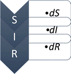
Figure 1 Diagram of SIR model following the solutions of the differential equations to find the solution.
S(t) is the susceptible, I(t) the infected, and R(t) the recovered people at the time t. β is the constant that represents the contact rate and γ is the inverse of the average infectious period. N is the total population in the function of the other variables
SEIR Model
The SEIR method was modeled with the Epidemic Calculator program obtained from https://rb.gy/4qguan. The SEIR model can analyse infectious diseases where the people have an exposed period to the virus and can transmit the infection to the rest of the population. The epidemic SEIR model diagram is shown in Figure 2 and its equations in (6), (7), (8), (9).
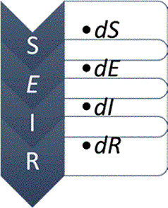
Figure 2 Diagram of the SEIR model following the solution of the differential equations to find the solution.
S, I, and R are the same values of susceptible, S(t), infected, I(t), and recovery, R(t), people respectively with exposed E(t) in the function of time.
The exposed people E(t) into the SEIR model is constituted by two classes, the first one is related to people that do not have the infection yet, and the second is the persons that change to recovered status. The new population number is:
RESULTS AND DISCUSSION
The nine countries were chosen as a representation from Europe of those where a decrease of SARS-CoV-2 infection was identified. The disease in the early stages in the American continent was evaluated in four of the bigger countries to compare with the European countries. Brazil was discarded because the model SIR cannot be calculated for having many infections peaks. Figure 3 shows the number of real infected, death, and recovered people of COVID-19 disease obtained from https://data.humdata.org and https://covid19info.live/. These data show that the epidemic is growing, the US has the greatest number of infected people of the nine countries studied followed by Spain, Italy, France, United Kingdom, Germany, Canada, Mexico, and Argentina as shown in Figure 3.

Figure 3 Representation of the real number of a) infected, b) deaths, and c) recovered people with the COVID-19 infection from the beginning of the SARS-CoV-2 virus propagation until 4/27/2020 of nine countries in this research.
In this period Argentina is the country with less infected people. However, the US occupies first place in recovered people followed by Spain, Germany, Italy, France, Canada, Mexico, UK, and Argentina. In the European countries, the disease exists since a few weeks ago and it is just beginning in Latin America. Most deaths were in the US followed by Italy, Spain, France, UK, Germany, Canada, Mexico, and Argentina. To study the propagation of the disease in the countries, one first statistics approximation to predict the maximum of infected cases of COVID-19 disease was realized with the coronavirus tracker, country modeling version 2.6.7 by Joshua McGee from MathWorks. This function was used to evaluate all the variables needed to solve the equations and calculate the values of the A, B, C variables of the Equation (1) with the real data obtained from https://data.humdata.org of the nine countries studied. The simulation is shown in Figure 4, and the values of the constants A, B, C, and the solutions of the total cases predicted with this model are described in Table 1. The US has a major number of infected people with 1,098,508 sick persons. Argentina on the other hand shows the less sick people with 4,860 predicted confirmed cases.
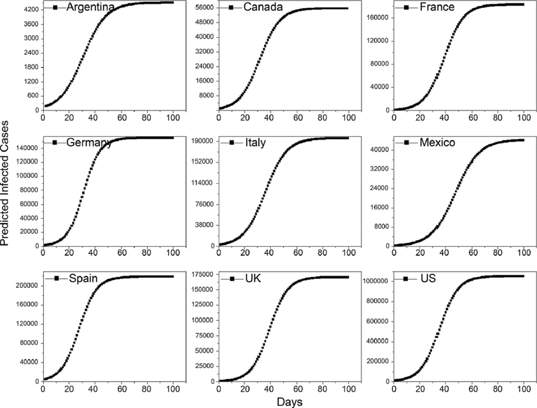
Figure 4 The predicted infected cases of SARS-CoV-2 using the nonlinear modelling in Argentina, Canada, France, Germany, Italy, Mexico, Spain, UK and US.
Table 1 Confirmed total cases obtained solving the nonlinear Equation 1.
| Nonlinear regression simulation1 | ||||
|---|---|---|---|---|
| Country | A | B | C | Confirmed Total Cases |
| Argentina | 4,506.9 | 0.11097 | 30.922 | 4,504 |
| Canada | 55,765 | 0.12697 | 56.777 | 55,755 |
| France | 1.8275e5 | 0.13328 | 181.43 | 182,696 |
| Germany | 1.5488e5 | 0.15681 | 133.67 | 154,876 |
| Italy | 1.9566e5 | 0.11976 | 75.568 | 195,566 |
| Mexico | 44,292 | 0.10814 | 170.35 | 44,140 |
| Spain | 2.1922e5 | 0.14474 | 54.74 | 219,213 |
| United Kingdom |
1.7088e5 | 0.14075 | 252.4 | 170,846 |
| United States |
1.0527e6 | 0.1384 | 132.43 | 1.05256E6 |
Table 2 shows the projected deaths in the nine countries using the nonlinear regression model. For the US the model predicts the most quantity of deaths with 59,929 followed by Italy with 26,373, France with 25,790, the UK with 23,067, Spain with 22,432, Germany with 5,866, Mexico with 4,077, Canada with 3,148 and for Argentina the model predicts the smallest value with 222.
Table 2 Projected deaths using the nonlinear regression simulation.
| Nonlinear regression simulation1 | |
|---|---|
| Country | Projected Deaths |
| Argentina | 222 |
| Canada | 3,148 |
| France | 25,790 |
| Germany | 5,866 |
| Italy | 26,373 |
| Mexico | 4,077 |
| Spain | 22,432 |
| United Kingdom | 23,067 |
| United States | 59,929 |
Results using the SIR epidemic model program downloaded from MathWorks are shown in Figure 5 for each country. The total of daily predicted cases with this model are adjusted for Canada, France, Germany, Italy, Mexico, and the UK, but not for Argentina, Spain, and the US. This model shows that Argentina, Canada, France, Germany, Italy, Spain, UK, and the US are decreasing in the number of total daily cases while France, Germany, Italy, and Spain are near to the final cases predicted. Mexico is the only one that is growing the disease. The tendency of cases predicted is near to close in the countries where the COVID-19 started such as France, Germany, Italy, and Spain.
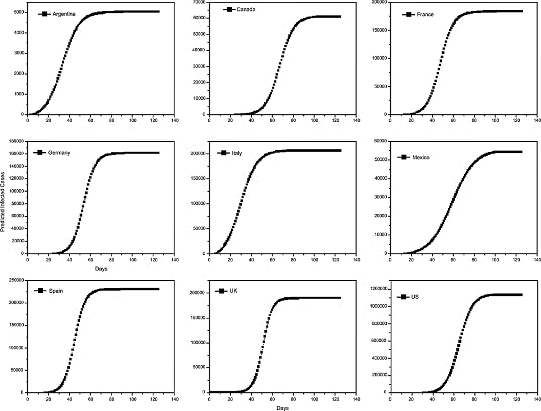
Figure 5 The predicted infected cases of SARS-CoV-2 using the SIR epidemic model using fitVirusCV19v3 (COVID-19 SIR Model) by Joshua McGee from MathWorks in a) Argentina, b) Canada, c) France, d) Germany, e) Italy, f) Mexico, g) Spain, h) the UK and i) the US.
The fitviruscv19v3-covid-19-sir-model function (from MathWorks page, https://rb.gy/qblldl) was also used to calculate the values of the contact rate β, the inverse of the average infectious period γ and the basic reproduction number Ro, required to predict the total projected confirmed cases of COVID-19 and these data were used to evaluate both epidemic models (SIR and SEIR). The data obtained from the software are shown in Table 3.
Table 3 SIR epidemic model simulation values1.
| SIR epidemic model simulation1 | ||||||
|---|---|---|---|---|---|---|
| Country | % Deaths2 | % Infected2 | β | γ | Ro | Population3 |
| Argentina | 4.9 | 66.6 | 0.641 | 0.541 | 1.182 | 44e6 |
| Canada | 5.7 | 57.5 | 0.298 | 0.166 | 1.792 | 37e6 |
| France | 14 | 58.1 | 1.849 | 1.714 | 1.079 | 66e6 |
| Germany | 3.9 | 24 | 0.307 | 0.136 | 2.25 | 83e6 |
| Italy | 13.5 | 53.1 | 0.26 | 0.135 | 1.928 | 60e6 |
| Mexico | 9.2 | 32.3 | 0.239 | 0.132 | 1.81 | 129e6 |
| Spain | 10 | 36 | 0.29 | 0.133 | 2.18 | 46e6 |
| United Kingdom |
13.3 | 83.9 | 0.303 | 0.16 | 1.896 | 66e6 |
| United States |
5.7 | 80.5 | 0.313 | 0.167 | 1.868 | 327e6 |
1https://la.mathworks.com/matlabcentral/fileexchange/74676-fitviruscv19v3-covid-19-sir-model
The data obtained for β, γ and Ro with the SIR model were used in the simulator of SEIR epidemic model in http://gabgoh.github.io/COVID/index.html to obtain the graphs of Figure 6 to predict the projected infected cases in Argentina, Canada, France, Germany, Italy, Mexico, Spain, UK, and the US. Table 4 shows the data of the variables obtained with the SEIR epidemic model to make the predictions.
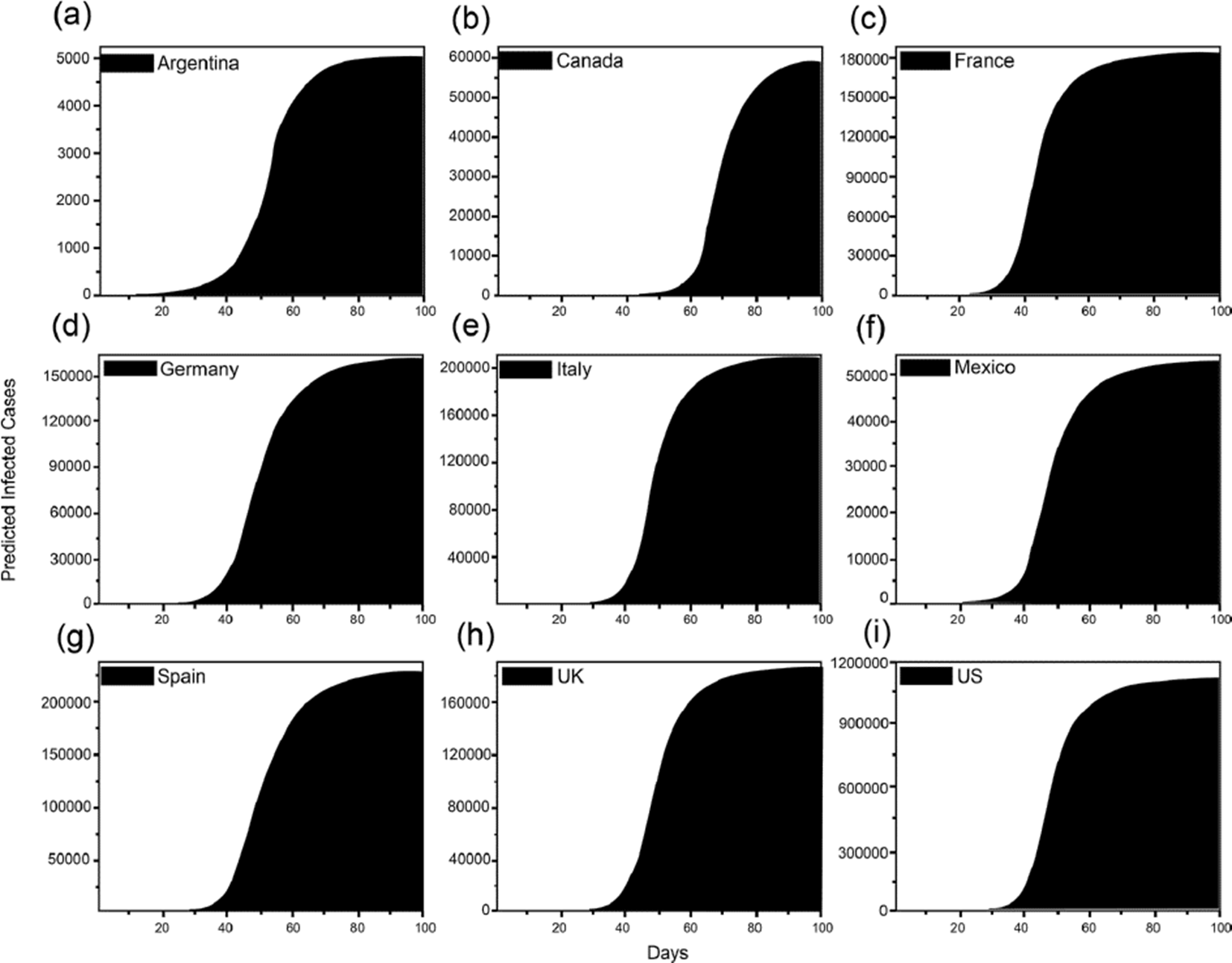
Figure 6 The predicted infected cases of SARS-CoV-2 using the SEIR epidemic calculator from the beginning of the COVID-19 infection until 4/27/2020 in a) Argentina, b) Canada, c) France, d) Germany, e) Italy, f) Mexico, g) Spain, h) the UK and i) the US.
Table 4 SEIR epidemic model simulation1.
| SEIR epidemic model simulation1 | |||||
|---|---|---|---|---|---|
| Country | Population | Ro | Β | κ | α |
| Argentina | 44e6 | 1.182 | 0.22 | 2.5 | 0.44 |
| Canada | 37e6 | 1.792 | 0.21 | 0.21 | 0.43 |
| France | 66e6 | 1.079 | 0.86 | 6.25 | 1.72 |
| Germany | 83e6 | 2.25 | 0.15 | 0.17 | 0.29 |
| Italy | 60e6 | 1.928 | 0.14 | 0.28 | 0.29 |
| Mexico | 129e6 | 1.81 | 0.10 | 0.45 | 0.20 |
| Spain | 46e6 | 2.18 | 0.11 | 0.25 | 0.22 |
| United Kingdom |
66e6 | 1.896 | 0.11 | 0.41 | 0.22 |
| United States |
327e6 | 1.868 | 0.14 | 0.43 | 0.29 |
Table 4 shows values of the contact rate β, the mean exposed period 1/κ, the rate at a recovery of disease γ =1/α, where α represents the infectious period, and basic reproduction number Ro calculated with the SEIR model in the epidemic calculator modeling obtained in http://gabgoh.github.io/COVID/index.html.
Table 5 shows the results predicted using the three models: the nonlinear regression, the SIR and SEIR epidemic model, and the average of the total projected confirmed cases of COVID-19 in the nine studied countries.
Table 5 The total confirmed cases of COVID-19 in the nine countries studied.
| Total Projected Confirmed Cases | ||||
|---|---|---|---|---|
| Country | Nonlinear regression
simulation |
SIR epidemic model simulation |
SEIR epidemic model simulation |
Average |
| Argentina | 4,504 | 5,000 | 5,076 | 4,860 |
| Canada | 55,755 | 60,053 | 60,280 | 58,696 |
| France | 182,696 | 184,286 | 184,711 | 183,897 |
| Germany | 154,876 | 161,426 | 161,921 | 159,407 |
| Italy | 195,566 | 205,483 | 207,812 | 202,953 |
| Mexico | 44,140 | 53,462 | 53,496 | 50,366 |
| Spain | 219,213 | 229,050 | 231,901 | 226,721 |
| United Kingdom |
170,846 | 187,819 | 187,905 | 182,190 |
| United States |
1.05256E6 | 1.12119e6 | 1,121,774 | 1,098,508 |
In Figure 7 data are plotted and show that United States has the greatest average number of cases with 1,098,508 followed by Spain with 226,721, Italy with 202,953, France with 183,897 United Kingdom with 182,190, Germany with 159,407, Canada with 58,696, Mexico with 50,366, and Argentina with 4,860 in average.
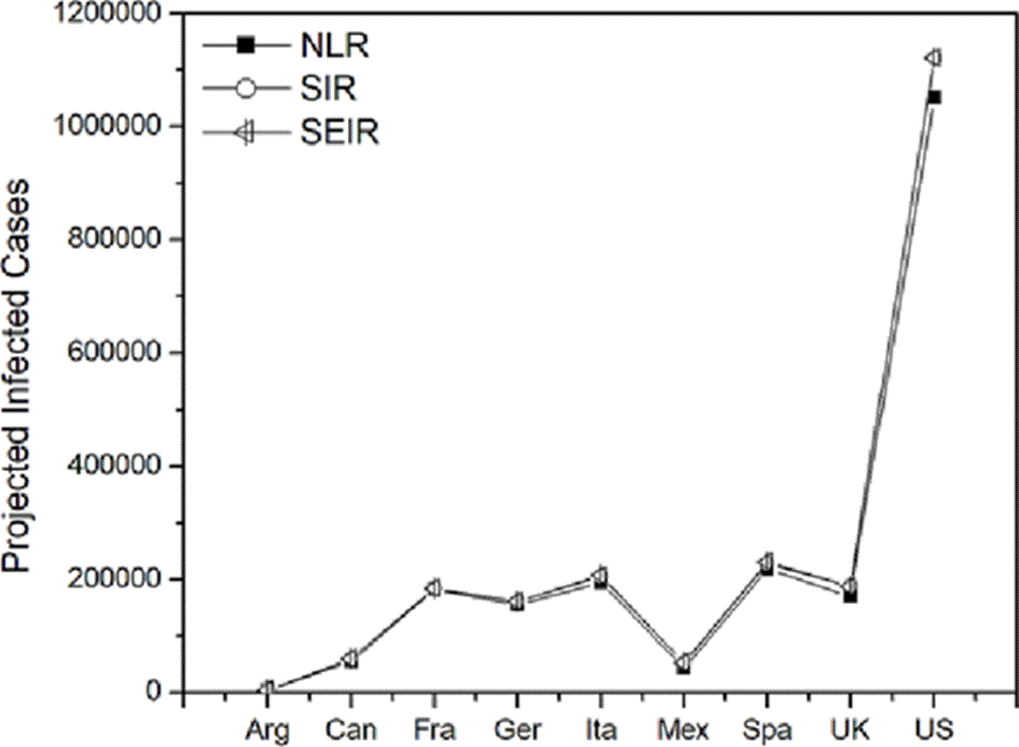
Figure 7 Comparison of projected infected cases between the three models studied: nonlinear regression, SIR and SEIR epidemic model of the COVID-19 infection from the beginning of the SARS-CoV-2 virus propagation until 4/27/2020 of nine countries.
Like the number of infected people in different countries is not equivalent, the comparison between the three methods is not balanced, besides to find if the methods have a significant difference around the means of nonlinear regression, SIR and SEIR method one-way ANOVA is used to compare them.
One-way ANOVA study is showed in Table 6. As can be seen from the data the three methods mean are not significantly different.
Table 6 One-way ANOVA1 of the nonlinear regression, SIR, and SEIR epidemic model.
| One-way ANOVA | |||
|---|---|---|---|
| Data | Mean | Variance | N |
| NLR | 231,128.44 | 1.00629E11 | 9 |
| SIR | 245,307.66 | 1.13995E11 | 9 |
| SEIR | 246,097.33 | 1.14054E11 | 9 |
| F=0.00583 | |||
| P=0.99419 | |||
1At the 0.05 level
Other studies have modeled SARS-COV 2, applying different models including nonlinear regression, SIR, and SEIR epidemic models [7] [11] [12] [13] [14] [15] [18] [19] [20], but they have no compared the results obtained among them as it is done in this paper.
Thus, if the results obtained are considered with the SIR model, then it can be observed that the REAL cases fit very well with the SIMULATED ones. When the SEIR model simulation is carried out, there are no variations, since there is no effect to take into account "for this virus" with the asymptomatic people who were exposed, E (t), since they do not generate significant variations for the model. Then the two models present similar results, which is what is being obtained in the one-way ANOVA. Therefore, it could be said from this comparison, that the SIR model is sufficient to predict the rest of the pandemic. Additionally, it is possible to see that for the SEIR model, there is a little effect when asymptomatic exposed people to this virus are taken into account, it can be assumed that there is no effect because they are only infecting the others, and since they do not present symptoms, the SEIR model considers them healthy until they are already part of the group of infected, I (t), so the results are similar.
On the other hand, the linear regression model is only making an adjustment with the real data and only allows predicting the maximum value of possible cases of infected people, but the SIR model can predict the daily cases and their decrease per day and predict how long the infection period can last.
CONCLUSIONS
The nine countries studied concerning the projected infected cases by SARS-CoV-2 using nonlinear regression method, SIR and SEIR epidemic model simulation, do no show equal predicted values, but those are not statistically different. It is confirmed by one-way ANOVA analysis. The above could mean that initially any method can be used to model the pandemic course.
These methods can be a first approximation and could help health professionals, not only the epidemiologist, to make decisions with a general point of view of a pandemic evolution.


 nueva página del texto (beta)


