1 Introduction
Cracks are the more typical kind of pavement affectations which can significantly decrease road safety and performance. This type of pavement deterioration is mainly caused by load traffic and some weather conditions. Early crack detection is a crucial step for road maintenance and therefore for enhancing road security.
Formerly, crack detection was carried out by manually segmenting cracked images, but this hand-operated approach is considered tardy, un-safe, non-objective and labor-intensive [3,15]. In recent years, this activity has been carried out in a faster, safer and reliable way. So automatic pavement crack has captured the attention of the computer vision community, proposing a great quantity of algorithms for this task.
A variety of approaches base their operations on setting a threshold value supposing that cracked pixels are darker than their neighbor pixels [13,8], Edge detection [24] considers that a crack is a remarcable point on the pavement. The main disadvantage about these methods is that they strongly depend on the illumination context and have just a local view of the problem.
There have been many recent methods focused on solving this problem (e.g., [1,11,16] used minimal path based methods (MPBM), [4,23,6,2,17] employed Convolutional Neural Networks (CNN), and [19] utilized tree architectures).
Automatic pavement crack segmentation remains a very challenging problem due to crack texture variety, different type of noises, also shadows, leafs, oil and water spots, large variability of crack forms, etc. Literature has reported many related works addressed to automatically detecting pavement cracks. However, most of these works have achieved low classification percentages, or have used non-public datasets which complicate establishing a comparison point between previous and new methodologies.
For solving this problem, we employ two well-known datasets: CFD and AigleRN, which are used in a considerable amount of recently published articles that propose new crack segmentation techniques.
In this work, we employ U-Net architecture as a base, which is a Fully Convolutional Neural Networks (FCNNs) typically utilized for biomedical images segmentation [18], and propose two variants for automatic pavement crack detection. The main contributions of this research are:
We propose two U-Net based network variations for automatic pavement crack detection.
We perform several experiments to demonstrate that the proposed architectures outperform the state-of-the-art for automatic pavement crack detection using two public and well-known challenging datasets: CFD and AigleRN.
We provide the code to segment cracks which also works for other datasets, https://github.com/RyM-CIC/Crack-segmentation.
Remaining sections are organized as follows: Section 2 gives specific details about FCNN and U-Net architecture and the proposed architectures for automatic pavement crack detection. Section 3 presents the related work used to resolve this problematic, and the two most outstanding researches related to ours, together with an understandable description of each. Section 4 discusses the datasets and the experimental results using two well-defined databases that can be compared and tested. In Section 5, we provide our conclusions and make some recommendations for future work.
2 Related Work
Related researches have tested the performance of many traditional algorithms and methodologies for pavement crack detection. In this section, we describe previous works that have performed crack segmentation using different methodologies, and two works that represents the state-of-the-art for automatic pavement crack detection using CDF and AigleRN datasets.
In [10,7] the authors use the idea that affected areas by cracks are darker than their surroundings and this methods obtains good performances. However, they are very susceptible to thinks such as shadows, water spots and oil, affecting their efficiency in real environments. With the arrival of machine learning, new methodologies were proposed that present a great robustness to this type of problems, [8] uses artificial neural network models for the automatic detection and classification. However, this model cannot correctly classify cracks with poor continuity.
First, Shi et al. [19] employed random structured forests to automatically detect cracks, CrackForest. From our point of view, this technique is complex because it involves several procedures and algorithms.
From the training image patches, CrackForest starts by computing a great quantity of features (a mean value, a standard deviation matrix, two magnitude and eight orientation channels, gradient and oriented gradient information, and so on) to describe the tokens (segmentation masks). The second step is clustering the formed tokens by using random structured forest in order to form a crack detector. Due to the large collected quantity of features, the procedure gathers 32640 features. To reduce the vector dimensionality, 256 features are randomly chosen to train each split function and then apply PCA (Principal Component Analysis) to reduce from 256 into five dimensions. Then, dilation and erosion operations are performed to connect different cracks in the image. Lastly, classification methods such as SVM (Support Vector Machine) and kNN (k-Nearest Neighbor) are applied to distinguish cracked pixels from noises.
The main disadvantage of CrackForest is that it strongly depends on the extracted features to describe the cracks. Nonetheless, because of the large quantity of pavement conditions, it is very difficult to extract representative features for all types of pavements.
Fan et al. [4] used a CNN with structured prediction for automatic pavement crack detection. The network has nine layers: four convolutionals, two max-pooling and three Fully-Connected (FC). The proposed architecture extracts patches from the original images to analyze pixel per pixel individually. The network determines if the analyzed pixel is a crack or non-crack pixel by forming a probability map in the network output. Despite the proposed methodology being very robust, effective and slightly improving the performance achieved by Shi et al. [19], it consumes many computational resources and time because it makes a sweep of all the pixels by creating a patch per pixel of the image.
The main advantage about using our proposals is that they only employ one architecture and do not depend on other algorithms or methodologies. Moreover, they overcome the state-of-the-art for automatic pavement crack detection.
3 Fully Convolutional Neural Networks
3.1 Convolutional Neural Networks
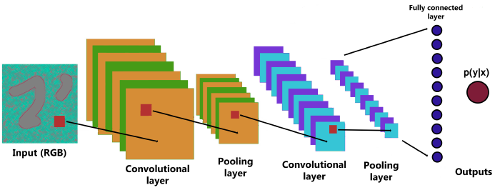
Typical convolutional classification nets [12,11,21] take sized inputs and produce non-spatial outputs. The fully connected layers of these nets result in spatial coordinates (Fig. 1). The resulting map is equivalent to the evaluation of the original image over all the possibilities. In order to obtain a segmentation it is necessary that these maps generate a h×w×d-sized output, so an adaptation in the last layers is necessary.

Fig. 1 Classification network composed of input (h×w×d), convolution, pooling and fully connected layers to result in a probability output
Fully Connected Neural Network (FCNN) operates over a input size of h×w and produces an output of corresponding spatial dimentions (it may be increased or reduced from the original image). These are powerful visual models that yield hierarchical characteristics of input images and have shown that by themselves, trained end to end, pixel to pixel, obtain better results than classical segmentation techniques [14] and for visual recognition problems [5,11].
A FCNN is a combination of operators such as convolutional layers, pooling layers, activation functions, upsamplings and so on. Each layer of data in FCNNs is a three-dimensional array of h×w×d size, where h and w are spatial dimensions, and d is the channel dimension (Fig. 2). The first layer is the raw image which has a dimension of h×w with d color channels.
Their classic components operate on local input regions and depend only on relative spatial coordinates expressed as xi,j for the data at location (i, j) in a layer, and yi,j the next layer connected, computed as:
where k is the kernel size, s is the stride, and ψks determines the type of layer:
-a matrix multiplication for convolution
-a spatial max for maxpooling
-an nonlinearity for activation function.
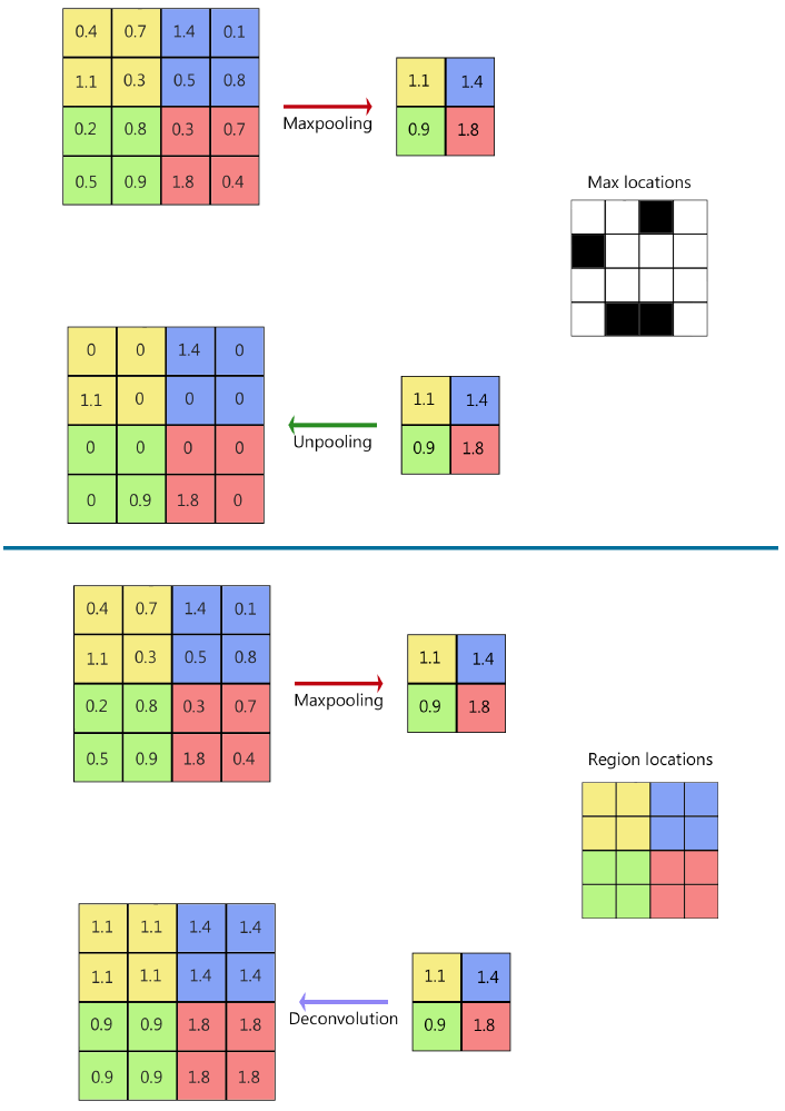
In a convolutional network, pooling is designed to filter noisy activations in lower layers by abstracting activations. It helps to classify by retaining robust activations in upper layers. However, spacial information is lost, which may be critical for precise localization in semantic segmentation. On the other hand, unpooling layers perform the opposed operation of pooling by reconstructing to the original size of activations [22]. So it records the locations of maximum activations selected in the pooling operation, and returns them to its original pooled location (Fig. 3).

Fig. 3 In upsampling methods, unpooling returns the original size of the filter filled with zeros in empty spaces recorded in max locations, deconvolution copy the same value in a region
The output of an unpooling layer is an enlarged activation map. In order to densify these activations, a deconvolution layer with multiple filters is used. Contrary to a convolutional layer, which is connected with multiple input activations within a filter window to a single activation, deconvolutional layers associate a single input activation to multiple outputs. Similar to a convolutional network, hierarchical deconvolutional layers are used to capture different levels of shape details.
3.2 U-Net
In 2015, Olaf Ronneberger et al. [18] proposed U-Net as a new type of FCNN which uses information from previous convolutional layers to segment biomedical images with high precision.
It consists of a contracting path (left side) and an expansive path (right side). The contracting path follows the typical architecture of a convolutional network. It consists of the repeated application of two 3x3 convolutions (unpadded convolutions), each followed by a rectified linear unit (ReLU) and a 2x2 max pooling operation with stride 2 for downsampling. At each downsampling step it double the number of feature channels.
Every step in the expansive path consists of an upsampling of the feature map followed by a 2x2 convolution ("up-convolution") that halves the number of feature channels, a concatenation with the correspondingly cropped feature map from the contracting path, and two 3x3 convolutions, each followed by a ReLU. The cropping is necessary due to the loss of border pixels in every convolution. At the final layer a 1x1 convolution is used to map each 64- component feature vector to the desired number of classes.
In addition to presenting a better performance than the state-of-the-art algorithms for segmenting biomedical images, it is fast and can be implemented with least training data.
In this paper, we use U-Net (named as U-Net-A). And we propose two variant of U-Net-A: U-Net-B and U-Net-C, by changing the architecture depth for automatic pavement crack segmentation. U-Net-A has 23 convolutional layers, U-Net-B has 11 and U-Net-C has 7 as shown in Fig. 4.
The purpose of modifying the architecture of the U-Net is to verify if architectures with less depth can obtain similar or better results than the original and thus reduce the processing time, which is very important in embedded systems, or in real time systems.
All U-Net architectures consist of convolutions of 3x3, 2x2,1x1, max pooling of 2x2 and steps of concatenation. RGB (red/green/blue) images of 480x320x3 pixels are used as network inputs.
Internal convolution layers use 'ReLu' function as an activation function defined as:
The last convolutional output layer uses 'Softmax' function (Equation 3) to output the image of size equal to the entry where the cracks are segmented:
4 Experiments
In this section, we evaluate and analyze the performance of the U-Net-A variants: U-Net-B and U-Net-C for automatic pavement crack segmentation with two challenging and well-known datasets.
We also compare our results with other works that represent the state-of-the-art in the segmentation of cracks, using the same metrics, the same databases and implement a variant of VGG16 by using the weights obtained in the training with ImageNet also adapting a series of deconvolutions to its final layers that allow obtaining a binary image representing the segmentations.
All experiments were conducted on a desktop machine with Intel-7i-2600 processor, 8G RAM and a GTX 980iGPU using libraries of Tensorflow and Keras, 'Binary cross entropy' is used as a loss function, and an ADAM optimizer [9], with a number of epochs of 300 for all cases. The source code can be found in [https://github.com/RyM-CIC/Crack-segmentation].
4.1 Datasets
In literature, we find a big variety of algorithms and procedures for automatic pavement crack detection. Nevertheless, most employ non-public datasets, which complicate establishing a comparison point between previous and new methodologies. For this reason, we used two well-known datasets: CFD and AigleRN.
CFD [19] is a common benchmark composed of 118 RGB cracked images with a 320x480 pixel size. These images were collected by using an iPhone 5 in Beijing, China. Each image has a hand labeled ground truth, and some typical perturbations such as different illumination types, water and oil stains and some shade types. For experiments, we employed 100 images for training and the rest for testing.
The other used dataset was AigleRN [1]. This consists of a challenging benchmark of 38 gray-scale images with a 991x462 pixel size taken from different French cracked pavements with intense crack texture inhomogeneity. This dataset is utilized to test the trained FCNNs.
Training and testing images did not have any kind of pre-processing and ground true labels were converted into RGB images with binary values.
4.2 Evaluation Procedure and Metrics
In order to evaluate the performance of the proposed architectures and compare it with other published articles that have worked with these datasets, we calculate the F1-score. F1-score is defined as the armonic mean between precision and recall, defined as:
where Pr is the precision of the architectures, TP is the correct segmentation of a pixel as part of the cracked pavement, FP is a positive false segmentation of a pixel as a part of cracked pavement and FN is a false negative, Re is the recall and F1 is a harmonic mean between precision and recall. For all experiments, we consider true positive pixels those which are no more than five pixels away from the ground true label pixels.
4.3 Results and Discussion
For training the FCNNs, 100 images of the CFD dataset with their respective manual segmented labels were used. For testing, 18 images of CFD and AigleRN dataset were utilized, to guarantee that the models do not present overfitting and can be used in databases different from the one used as training, and even so they can segment the cracks in different types of pavements.
Table 1 shows the results obtained after training all the FCNNs.
Table 1 Summary of performance details of the different neural network structures
| Net | Time | Results (CFD Dataset) | |||
|---|---|---|---|---|---|
| Training | Test | Precision | Recall | F1 | |
| U-Net-A | 153.3 min | 0.162 s | 96.93% ± 0.96 | 93.45% ± 1.30 | 95.00% ± 0.55 |
| U-Net-B | 93.3 min | 0.066 s | 97.31% ± 0.28 | 94.28% ± 0.51 | 95.75% ± 0.22 |
| U-Net-C | 80 min | 0.046 s | 95.77% ± 0.64 | 82.42% ± 0.90 | 87.66% ± 0.76 |
In order to corroborate the F1-score in U-Net based CNNs, we performed a series of training test, obtaining the mean and standard deviation.
Results from the dataset CFD demonstrate that proposed FCNNs have an average precision higher than 95% and a best performance of 97.31% in U-Net-B, which means that the segmentation is mostly correct having less false positives. The U-Net-B recall presents the highest result with 94.28% and U-Net-C shows 82.42% which means that U-Net-C has a significant percentage of false negatives. F1 score shows that U-Net-B presents the best performance by segmenting the major part of the cracks correctly.
FCNNs require more training time as more convolutional layers are added. Similarly, the time to process an image increases up to 0.162 seconds in U-Net-A.
As can be seen, U-Net-C has a poor performance compared to the other two architectures, with a 1% lower precision than U-Net-A and U-Net-B, and up to 12% of less recall. So, this architecture is disregarded as a possibility of use in future comparisons.
After measuring the FCNNs performance with the same dataset used for training, we compare the proposed FCNNs with related works that use the same datasets, Table 2, shows different results using the CFD dataset as a training dataset, and CFD and AigleRN as the testing dataset.
Table 2 Performance summary in pavement cracks with different approaches
| Method | Training/Test | Pr | Re | F1 |
|---|---|---|---|---|
| U-Net-A | CFD/CFD | 96.93% | 93.45% | 95% |
| U-Net-B | CFD/CFD | 97.31% | 94.28% | 95.75% |
| Canny | CFD/CFD | 43.77% | 73.07% | 45.70% |
| Local thresholding | CFD/CFD | 77.27% | 82.74% | 74.18% |
| CrackForest | CFD/CFD | 95.75% | 95.62% | 95.68% |
| Fan et al. [4] | CFD/CFD | 91.19% | 94.81% | 92.44% |
| VGG16 Modfied | CFD/CFD | 92.78% | 87.09% | 89.26% |
| U-Net-A | CFD/AigleRN | 94.98% | 65.81% | 75.61% |
| U-Net-B | CFD/AigleRN | 93.51% | 82.90% | 87.33% |
| Canny | CFD/AigleRN | 19.89% | 67.53% | 28.81% |
| Local thresholding | CFD/AigleRN | 53.29% | 93.45% | 66.70% |
| CrackForest | CFD/AigleRN | 87.43% | 85.52% | 86.46% |
| Fan et al. [4] | CFD/AigleRN | 64.88% | 88.19% | 71.82% |
| VGG16 Modified | CFD/AigleRN | 91.24% | 51.92% | 64.34% |
We implement a modification to VGG16 [20], which is a well-known architecture for the treatment of images and their classification in order to observe their behavior in the binary segmentation, for which the architecture was modified by replacing the last output layers by convolutional layers that return a binarized image of equal size to the input image that represents the cracks in the pavement.
Results show that U-Net-B has the best performance when CFD is employed to train and test with a 95.75% of correct segmentation.
Analogous when AigleRN dataset is used to test results change, U-Net-A presents the best precision rate with a 94.98% and Local thresholding obtains the best recall percentage with 93.45% which means this algorithm is able to segment the major part of the pavement cracks. Furthermore, even when U-Net-Bdoes not present the best precision or recall results, it maintains a higher F1 score, showing it can segmentthe cracks in the pavement better.
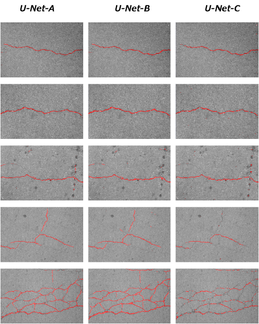
FCNNs results are shown in Figure 6 where cracks are represented in red color.

Fig. 6 Segmentation cracks with the different FCNNs. U-Net-B segments cracks without reducing the crack thinness and U-Net-C cannot recognize thin cracks
It is shown that U-Net-B obtains clearer segmentations of wide cracks. Moreover, it can identify thin cracks without continuity, and distinguishes between cracks, shadows and oil spots. U-Net-A has a worst performance than U-Net-B because it identifies some noises (oil spots and shadows) as cracks reducing the recall. And U-Net-C just identifies main cracks and cannot segment continuous lines.
5 Conclusions and Future Work
In this paper, we study FCNNs with three different depths to perform automatic pavement crack detection. Also, we compare our results with the algorithms that represent the-state-of-the-art for this task. The following are some significant findings:
- It has been shown that modified U-Net models can be successfully applied for solving automatic pavement crack segmentation problems proving a better performance than state-of-the-art methods.
- We proposed a FCNN based on U-Net, U-Net-B which improve the performance of previous works in segmentation of cracks in pavement, with a F1-score of 95.75% in the same dataset and a 87.33% with images from the other dataset, which is able to discriminate cracks from noises, and is faster than other architectures, using only 0.066 seconds to process an image.
- Analyzing different FCNNs types have shown that these perform better when they are trained and tested with the same dataset. Only deep architectures achieve good generalization when trained and tested with different datasets.
All these points show that we have presented three models able to automatically segment pavement cracks with a high F1-score and achieve good generalization by distinguishing among different types of outliers.
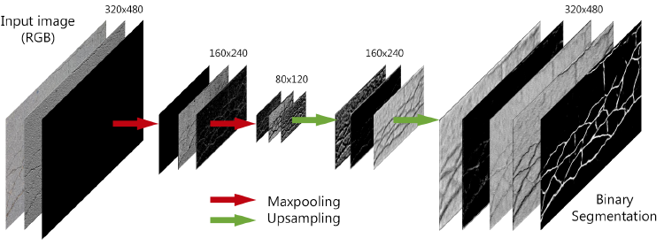
U-Net-B has a compact structure with a short processing time, which is composed of series of 3 convolutional layers followed by a maxpooling layer to reduce the size of the original image 75%. This is followed by a series of convolutions and upsampling layers, concatenated with their correspondent in the encoder part.
As shown in Fig. 7 the internal layers of U-Net-B process the raw image highlighting the cracks over the background to finally obtain a binary image.

Fig. 7 Visualization process of the U-Net-B model of the internal layers for the segmentation of cracks
Future work will focus on the analysis of binary images segmentation where these have much less region on interest to the rest of the image. This disproportion hinders the correct crack segmentation by reducing the crack continuity. As a consequence, the neural network achieves lower precision in the segmentation process.


 nueva página del texto (beta)


