


 nueva página del texto (beta)
 Inglés (pdf)
 Artículo en XML
 Referencias del artículo
 Enviar artículo por email
 Citado por SciELO
  Similares en
SciELO
Similares en
SciELO 
 Permalink
Introduction
The goal is the design
In civil construction practice, when projecting a building, the natural way of proceeding is that the architect proposes the forms, and the engineer runs the structural analysis based on those forms that, generally, have a previous structural design of the structure with a certain geometric rigidity. After a first analysis, any necessary modification to the original proposal needs the agreement of the parties in order to continue with the analysis until the project is definitively closed.
This iterative batch process, consisting of running the analysis, evaluating the results and modifying some parameters to finally arrive at an acceptable solution, is used by the majority of structural engineers and, usually, relies on heuristic rules where experience plays an important role (Figure 1a). However, it does not mean that the solution reached is the optimal one, nor that it cannot be improved in terms of the tensional behavior and the economy of the materials.

The fact is that, normally, engineers do not deal with the structural design as a primary goal (Norris et al., 1977). Instead, they focus on the structural analysis, which would be the final step of the design process, and carry out the calculus as a tool to check the fitness of shapes and dimensions to support the loads (Torroja, 2007).
A correct design of a structure implies its optimization, which means dealing with those methods that allow to choose the best possible solutions changing the transverse sections, geometric shape, topology or the material properties (Dimčić, 2011), (Figure 1b). It is not sufficient, therefore, to satisfy only resistance, stability and shape requirements of such an initial architectural proposal.
A general structural optimization (SO) problem can be defined as the search for the minimization of an objective function (f), under restrictions imposed by the design variables (which can be modified during the optimization process, as e.g. the shape or the material election), the state variables (related with the structural response) and the satisfaction of compatibility and equilibrium equations, which are expressed by means of state equation in linear analysis (Christensen & Klarbring, 2008).
In mathematical terms, a SO problem consists of obtaining those values of the n design variables
that minimize an objective function (weight, cost, etc.)
or more than one
under a set of r restrictions
that shall be taken into account in order to limit the search space and allow the solution to be feasible.
This requires the service of specific tools. However, since this kind of resources is still scarce and demands its development under an interdisciplinary approach between architects, engineers, and computer scientists (Jones, 2013; Ochsendorf, 2006), traditionally the optimization treatment has been reserved for the academic world.
There are many analysis tools in the market, but scarce ones to achieve good structural forms (Ochsendorf, 2006, 2012). In practice, engineers normally use classic structural analysis software for design purposes (Clune, 2010). However, this does not guarantee optimal solutions, or something close to them. As the structural performance depends on geometry, that focus will lead to structures of low efficiency (Danhaive & Mueller, 2015).
This fact is clearly evident in plane and space trusses, structural types widely used in industrial sheds, sports pavilions, among others, which have a significant incidence in the final construction cost.
In consequence, faced with the query of how to resolve the problem of achieving optimized designs for trusses, with efficiency and economy of materials, new streams of structural engineering seek optimization by means of parametric design and evolutive computing.
Parametric design with visual programming and genetic algorithms: A suitable and promising path
The basis of parametric design comprises a set of digital tools that allow the user to generate geometries on the basis of the definition of a family of initial parameters and the programming of the formal relations between them (Salcedo, 2012).
At present, parametric design software packages operating with visual programming, such as Grasshopper (Robert McNeel & Associates, 2015b), which run inside the geometric modeling software Rhinoceros (Robert McNeel & Associates, 2015c), have paved the way significantly for structural engineers to develop their own algorithms for the modeling and resolution of practical cases of different complexity within their professional expertise.
Visual programming has become a powerful and accessible tool to provide a versatile and simple language that does not require prior programming knowledge to generate the algorithm to solve problematic situations (Danhaive & Mueller, 2015).
The aforementioned software, complemented with structural analysis plug-ins by means of finite elements, and the implementation of evolutionary methods of optimization by means of genetic algorithms (GAs), make it possible to reach structurally efficient shapes with minimization of materials.
The GA optimization technique produces a range of possible optimal solutions, based on objective functions that define the design criteria. Likewise, the parametric design allows the introduction of a significant number of variables, making it possible to evaluate a large number of geometric configurations with the same algorithm. These new computer tools allow the unification of engineering design processes and the achievement of structural shapes, both free and complex, as well as precise and efficient (Maltagliatti, 2016).
AIM
The aim of this work is to present an algorithm developed by visual programming, for the optimization of the sections, shape and topology of plane trusses, taking as an example its application to a real structure, and highlighting the advantages that the use of this computer resource provides for the professional work of structural engineers, allowing them to develop their own algorithms without the need of previous knowledge of programming.
Methodology
Algorithm description
By means of Grasshopper, version 0.9.0076, an algorithm was developed by the authors for the optimization of plane trusses in relation to their own weight, which makes it possible to choose between three typologies: Howe, Pratt or Warren. The boundary conditions (supports, loads), the input parameters (material, section library) and other restraints are introduced from Karamba, version 1.1.0 (Preisinger C. and Bollinger-Grohmann-Schneider ZT GmbH, 2015), a parametric software of structural analysis by finite element method that operates as a Grasshopper plug-in and that, in addition to providing the structural responses, allows the optimization of the sections of each bar through an iterative process of stresses and displacements control.
The optimal distribution of the material in bars structures (topological optimization) is given by the search for the best interconnectivity among its members (Hultman, 2010) so that during the resolution process the removal of some of them takes place (Christensen & Klarbring, 2008). When it lacks control, this type of optimization generally leads to structures of great efficiency but very difficult to materialize. Hence, to achieve a tool that can be applied in professional practice it is necessary to establish design limits. For this reason, the algorithm developed does not generate free form structures but is limited to the indicated typologies (Bonelli & Begliardo, 2016).
Through Galapagos (Robert McNeel & Associates, 2015a), an evolutionary solver by genetic algorithms that operates as an add-on of Grasshopper modifying the design variables within established domains, an initial population of possible solutions (individuals) is created. This is then subjected to selection, crossing and mutation processes, for which an evaluating function is used to determine which individuals are the fittest that will survive and which will be discarded. This evaluator, called fitness, is the weight of the truss. The lower the weight, the greater the aptitude, and vice versa.
Through the repetition of the selection, combination, and mutation process of individuals, new generations evolve towards the individual with the best fitness. When an individual becomes stable during n generations, without the appearance of a better new one, a global optimum or an individual near to it has been obtained, and the process stops. As a consequence of this, the cross-section size of each bar, the shape, and the truss topology (expressed in the gaps number) have been optimized.
The screen image of Figure 2 shows the assembly of the aforementioned software in the algorithm under the Rhinoceros (version 5.0) modeling software environment.

Design variables
The variable parameters constitute the degrees of freedom of the problem that allows for the definition of the structural geometry. A usual way of expressing them has been indicated in (1). Each of them has a domain defined by a maximum value and a minimum value.
Figure 3 defines the variable parameters used in the algorithm, while Figure 4 shows, on the left, its definition in Grasshopper based on sliders that allow variability. On the right, the domain predefined by the user is shown to establish the length of the truss to be optimized, and the adopted value of the clear span.


Each modification of a variable creates a new structure, and the totality of the combinations establishes the solution set, that is, the search space of the optimal truss.
The objective function
In structural engineering, this function usually describes a minimization problem. In this case, what has been sought is the structure of minimum weight w(x), as it is a decisive factor in its final cost, and it is associated with a lower consumption of material.
Assuming that each i bar has a straight direction and constant cross-sectional area A i in its entire length l i , on the basis of (2), the result is:
Where:
γ i being the specific weight of the material, which is usually the same for the entire structure.
Imposed restrictions
In addition to the restrictions imposed by the design variables, the algorithm establishes behavioral limitations on the state variables and the verification of the state equation:
a) Behavioral restrictions: The axial load Pi in each bar i, both in tension and compression, must not exceed the maximum value Pu i that can resist the material, nor suffer from problems of local instability.
Pu i is determined by the yield stress Fy i of the material. Assuming that it is unique, then
The deflection δ at any point in the structure must not exceed a predefined δ max value or a value set by regulation
where L is the clear span of the structure and k is the deflection factor which, for trusses, usually takes a value between 200 ≤ k ≤ 300.
b) Equilibrium restrictions: State equation in the linear static analysis must be verified
where:
K = |
rigidity matrix of the structure |
u = |
vector of the unknown nodal displacements |
P = |
vector of external forces |
That is to say, the optimal structure of lower weight will be obtained from the point of view of resistance, and that is the one that allows the maximum use of the material, fulfilling the equilibrium and compatibility conditions given by (10) (Gil & Andreu, 1999).
Applied standards
The algorithm implements argentine standards (INTI-CIRSOC Regulations and specific IRAM Standards), in addition to Karamba's own library of sections. However, the addition of any other regulations is feasible, requiring the introduction of simple modifications.
Example
As an example of application to a real case, a Howe truss of 20 m clear span corresponding to a built industrial shed located in the central region of Argentina (Figure 5) was taken for analysis and comparison. The structural engineer analyzed it as a simply supported beam leaning on two columns.

However, in the building site, the supports were welded to columns, generating boundary conditions that modified the internal forces in truss members. The following are the constructive details:
Bars composed of cold-formed C sections (CFCS).
Heights: 0.50 m (lateral edge); 1.00 m (central).
Loads types: dead load (DL), imposed loads (IL) and wind loads (WL).
Idealized supports for analysis: roller support-hinged support (isostatic).
Materialization of supports on site: fixed (welded) on columns.
Truss´s weight (considering only profiles): 4.473 kN.
Through the application of the developed algorithm, the optimal design (weight minimization) of the truss was sought for the isostatic condition variant applied in the idealized model of the original structure and, additionally, for three more options of external supports, which are indicated in Table 1 as Cases 1 to 4. In all of them, the response was evaluated for the profile classes CFCS and CHS (circular hollow section).
Table 1: Analyzed cases (Howe type)
| Supports | Degree of redundancy | Profile | ||
|---|---|---|---|---|
| Case 1 | R-H | 0 (Isostatic) | CFCS | CHS |
| Case 2 | H-H | 1 (Hyperstatic) | CFCS | CHS |
| Case 3 | H-F | 2 (Hyperstatic) | CFCS | CHS |
| Case 4 | F-F | 3 (Hyperstatic) | CFCS | CHS |
Notations: R (roller); H (hinged); F (fixed)
CFCS (Cold-formed C section); CHS (circular hollow section)
Case 1 (CFCS) is similar to the idealized model in the constructed structure, and Case 4 (CFCS) is the one that most resembles the one materialized on the building site.
Argentina structural safety regulations were applied (CIRSOC, 2018), considering all combinations of loads prescribed for the region where the structure was built, with the dead weight (D), imposed loads (IL), wind loads (WL), concentrated loads (P) and thermal variation (ΔT). The Argentine Structural Security Regulations, second generation, are based on US codes. In particular, in the area of metallic structures, the rules of the AISC (American Institute of Steel Construction) are applied.
By default, the algorithm uses F-24 steel (equivalent to ASTM A36), although it can be modified. According to the regulations, δ max = L / 300 was adopted for the design.
In relation to the cross-sections, in addition to those included in Karamba, there is a library of steel profiles according to the standards of the Instituto Argentino de Normalización (IRAM, 2018), which makes it possible to include other standards if necessary by means of the addition of a spreadsheet.
On the basis of the clear span of the original truss, Table 2 indicates the numeric domain of the geometrical design variables applied to the algorithm.
Table 2: Parameters domains
| Design variables | Mini-mum | Maxi-mum | Observations |
|---|---|---|---|
| Left end-post height (hi) | 0.00 m | 1.00 m | Floor level minimum distance: 5.50 m |
| Right end-post height (hd) | 0.00 m | 1.00 m | Floor level minimum distance: 5.50 m |
| Left edge elevation (Δ a ) | 0.00 m | 0.00 m | See Figure 6 |
| Left top-chord height (Δ 1 ) | 0.50 m | 3.00 m | See Figure 6 |
| Left bottom-chord height (Δ 2 ) | -1.00 m | 4.00 m | Floor level minimum distance: 4.50 m |
| Maximun height (ht) | 0.00 m | 4.00 m | It is not a variable: ht = hi + Δ1- Δ2 |
| Nº of segments (gaps between vertical bars) | 16 | 24 | Purlins support distance: 0.80 m to 1.25 m |
| Profiles | CFCS - CHS | According to IRAM (2018) | |
Figure 6 illustrates the configuration of the geometric domain in which the search space for the best solution was delimited.

Results and discussion
In the runs analyzed, initial populations of 100 or 150 individuals were applied, with stopping criteria determined by the repetition of the most suitable genome for 100 generations, which led to a number comprised between 104 and 501 iterations, depending on the case.
Table 3 shows the results of the four cases analyzed (optimized design variables, weight, and L/ht ratio).
Table 3: Optimal design of the truss: values obtained
| Case 1 | Case 2 | Case 3 | Case 4 | |||||
|---|---|---|---|---|---|---|---|---|
| Design variables | CFCS | CHS | CFCS | CHS | CFCS | CHS | CFCS | CHS |
| Left end-post height (hi) | 0.85 | 0.98 | 0.90 | 0.99 | 0.98 | 1.00 | 1.00 | 0.94 |
| Right end-post height (hd) | 0.89 | 0.97 | 0.96 | 0.91 | 0.93 | 0.92 | 1.00 | 1.00 |
| Left top-chord height (Δ 1 ) | 0.50 | 0.54 | 1.95 | 1.93 | 1.60 | 1.76 | 2.08 | 2.03 |
| Left bottom-chord height (Δ 2 ) | -0.96 | -1.00 | 2.03 | 1.85 | 1.93 | 1.70 | 2.20 | 2.05 |
| Maximum height (ht) | 2.31 | 2.52 | 0.82 | 1.07 | 1.00 | 1.06 | 0.88 | 0.92 |
| Nº of segments | 16 | 18 | 18 | 22 | 20 | 22 | 16 | 24 |
| Clear span/ maximum height ratio (L/ht) | 8.6 | 7.9 | 24.4 | 18.7 | 20 | 18.9 | 22.7 | 21.7 |
| Weight (kN) | 2.744 | 2.247 | 2.079 | 1.545 | 2.198 | 1.661 | 2.231 | 1.715 |
Note: Units are in meters (m); Weights in kN (kilonewton)
For the simply supported condition (Case 1), the application of the developed algorithm led to a structural form that adapts to the law of bending moments (Figure 7), a conclusion also observed by Gil & Andreu (1999) for these cases.

Weights indicated in Table 3 refer to the full optimization, bar to bar, which for Case 1 (CFCS) leads to 8 different profiles, meaning a weight reduction close to 39 %. In practice, this presents drawbacks at the moment of constructing the truss, either due to difficulties in the assembly between one bar and the other, or because of the increase in the cost of labor. Normally, in these circumstances, the sections in chords, verticals, and diagonals are homogenized to gain constructive simplification. In this situation, adopting 4 different sections for the CFSC profile (one of them for the top chord, one for the bottom chord, one for both left and right end posts, and the fourth one for the rest of the inside members), for the cited variant that is compared, the reduction will be close to 25 %.
It is observed from the table that, in full optimization, for case 4 (CFCS) the reduction in weight would be 50 %, a fact that warns us about the importance of modeling a structure in the way that it effectively will be built (Bonelli & Begliardo, 2016).
Figure 8 shows schematically, and for comparative purposes, the external shape that the optimized truss takes depending on the type of external supports with which it is modeled. As it can be seen, there is a qualitative leap in the configuration when going from the isostatic case (Figure 8a) to the hyperstatic case since one additional restriction is incorporated (Figure 8b). This external form, substantially, does not change in the remaining two cases (Figures 8c and 8d). Likewise, from Table 3 it appears that the weight decreases significantly in the hyperstatic cases, being Case 2 (hinged-hinged supports) the one which leads to the lighter structure.
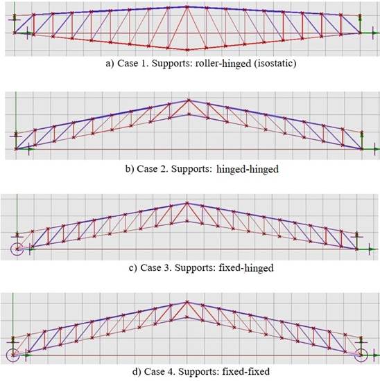
Figure 8: Schematics of the geometric shape that the truss takes, according to the kind of supports (Source: Bonelli & Begliardo (2016))
The topological optimization is shown in the number of cavities (16 for Case 1 (CFCS) compared), tending to the minimum possible value within the domain of the variation of the segments, which are pre-defined by the user as a design variable (16-24 according to Table 2). This will happen as long as the cross-sections of the library of available commercial profiles support the tension or compression loads to which the bars will be subject.
It also emerges from the aforementioned table that, in all cases, the use of SCH profiles leads to structures of lower weight than CFCS.
An output of the remarkable results of Karamba, in the framework of the search for sizing optimization, is that makes possible to know the advantages of the material bar to bar, in relation to its resistance capacity, a fact that allows structural engineers to regulate it according to their needs and restrictions.
As a complementary contribution to the information, Bonelli & Begliardo (2016) provide results for the four cases with the Pratt type truss variant.
Conclusions
An algorithm has been developed through visual programming for structural optimization of sizing, shape, and topology of plane trusses based on parametric design and genetic algorithms, with structural analysis resolution by the finite element method.
The field of structural optimization has been long questioned by engineers for its impracticalities in engineering practice (Clune, 2010). In this paper, paraphrasing this author, it has been demonstrated that the proposed resources are relevant and beneficial, and that they provide techniques to explore the design space in an optimal way, leading to structural designs that are feasible and can be built with less material and costs than structures designed by conventional software. Additionally, all this contributes to environmental sustainability, a premise that, as indicated by Ochsendorf (2012), should always be sought in the field of structures.
These resources allow structural engineers to customize algorithms in order to apply them to their current practice without the need for prior programming knowledge, making it possible to transfer advances in computer technology to professional practice and to extend the frontiers of academic applications.

