


 nueva página del texto (beta)
 Inglés (pdf)
 Artículo en XML
 Referencias del artículo
 Enviar artículo por email
 Citado por SciELO
  Similares en
SciELO
Similares en
SciELO 
 Permalink
Introduction
Deviations from the covered interest parity (CIP) across different foreign exchange markets, have been the norm in the aftermath of the financial crisis that erupted in the summer of 2007. These have been observed in the U.S. Dollar(USD)-Sterling, USD-Euro, and USD-Yen parities (Du et al., 2018). Deviations from the CIP in the USD-Mexican Peso (MXN) parity have also been observed. Notwithstanding the MXN is among the most traded currencies in the world (BIS, 2016), these deviations reveal apparent risk-less arbitrage opportunities.
The computation of deviations from CIP using USD-MXN future contracts, the yields on U.S. Treasury Bills and Mexico’s CETE, all for 1-month, displayed in Figure 1, shows the dates of the major shocks from the start of the financial crisis. In particular, the behaviour of these deviations is consistent with economic theory for the period January 2005-August 2007, since it is around zero. Major disruptions generated by severe financial stress events that unfolded in 2007 (e.g. the Bear Stearns buyout, the Lehman Brothers failure, the Troubled Asset Relief Program (TARP) approval within the U.S. Congress and the AIG’s bailout) are represented by extremely large deviations from the zero level. After the second half of 2009, the main sources of financial stress were the fragility of Europe’s banking sector and regulation introduced in the aftermath of the financial crisis.
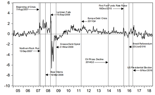
Source: Bloomberg.
Figure 1 Deviations from the CIP in percentage points for the period January 2005 to October 2018 computed using expression (2.4) below. Weekly averages of daily data.
A priori, it seems plausible the described events and regulation would cause funding liquidity in financial markets to fall. Reduced liquidity is defined as (i) the reduced availability of funds to undertake financial transactions in assets that are perceived riskier than those with the highest rate by rating agencies, and (ii) higher quality or quantity collateral demands. Given that underlying the CIP is a forward contract on the exchange rate, a further source of frictions might be found in the risk for the counterpart fulfilling their part of the contract. In this paper, the relative importance of reduced liquidity conditions in explaining deviations from CIP is tested and quantified.
The sequence of financial shocks from the summer of 2007 through the summer of 2012 and new regulation introduced since, suggests that there were two different sources of funding liquidity shocks: (1) U.S.-born, and (2) Europe-born. Their role in explaining deviations from the CIP is analysed accordingly. Shocks born in the U.S. are straightforward to relate to deviations from the CIP provided, among other reasons, that: (i) the U.S. economy is Mexican exports’ main destination, and so changes in the demand for goods made in Mexico affect the risk premium firms must pay when they are looking for sources of funding; (ii) the largest Mexican firms have access to credit valued in USD, which may be provided by U.S. based financial firms; and (iii) there is relatively high mobility of labour between the two economies, which changes the relative prices of production inputs, among them the interest rate.
Europe-born shocks are not as directly related to deviations from the CIP but they are still relevant for the analysis. The lack of a clear relationship between deviations in the CIP and Europe- born shocks, may bias analysts and economists’ judgement towards the claim that these shocks have only a short-run effect. An econometric-based answer to the latter statement is, however, absent in the literature.
To determine whether shocks in funding liquidity generate deviations from the CIP, and whether these deviations are persistent, a vector error-correction model (VECM) is used which includes the following variables: (i) the 1-month exchange rate forward premium; (ii) the yield on 1-month U.S. Treasuries; (iii) the yield on 1-month CETE; (iv) the LIBOR-OIS spread in USD; and (v) the analogous measure for Europe.1
The main findings are, first, apparent deviations from the CIP are persistent. Once the effects of funding liquidity shocks in the U.S. and Europe are included, however, an error-correcting relation- ship emerges (i.e. the CIP is satisfied). This means that arbitrage opportunities do not exist, once a measure to the costs of funding liquidity for the agents is included. Second, both the exchange rate forward premium and the U.S. interest rates adjust towards the error-correcting relationship that explains deviations from the CIP. Interestingly, the yield on 1-month Mexican CETE has its own stochastic trend, notwithstanding the strong relationship between U.S. and Mexico’s economies and the small open economy status of the latter. Third, a structural analysis confirms that the es- timated model is consistent with intuition relating the variables included in the VECM. Finally, it confirms that deviations from CIP are explained by changes in funding liquidity conditions. In particular, over time the relative importance of U.S. funding liquidity conditions is similar to that of deviations from CIP themselves. Moreover, contrary to what may be expected, the relationship between liquidity conditions in Europe and deviations from CIP is non-negligible.
To produce a survey of the vast literature around the CIP would require a great amount of space, but among the pioneers are Aliber (1973), Frenkel and Levich (1975), and Frenkel and Levich (1977). Indeed, up until the 2007 financial crisis, tests confirmed the validity of the CIP. These were made using high-frequency data sets (Akram et al., 2008, and Fong et al., 2010), panel data and single equation econometric techniques (Mancini-Griffoli and Ranaldo, 2011, Ivashina et al., 2015, Sushko et al., 2016, and Avdjiev et al., 2017), and time series multiple equation techniques (Clarida and Taylor, 1997, Shigeru and Shu, 2006, Roll et al., 2007, and Eichengreen et al., 2012). Cointegration techniques have also been used to determine if the CIP is satisfied (Peel and Taylor, 2002, and Sushko et al., 2016).
Since deviations from CIP in major foreign exchange markets have been the norm in the post 2007 crisis period, literature has turned its attention to find possible explanations. This has taken the form of omitted variables analysis, much in the same way the present paper does for an Emerging Market economy (Mancini-Griffoli and Ranaldo, 2011, Levich, 2012, Ivashina et al., 2015, Sushko et al., 2016, Liao, 2016, Borio et al., 2016, Avdjiev et al., 2017, Cenedese et al., 2017, and Du et al., 2018). More recently, attention has turned to bands-about the CIP and one-way arbitrage, as suggested by Levich (2017).
The CIP related to the USD-MXN parity is an interesting case to analyse since the financial crisis may be considered as an exogenous shock (i.e. not caused by Mexican macroeconomic outlook which at the time enjoyed sound macroeconomic indicators, and a sustainable current account deficit, IMF, 2007). The references for this foreign exchange market include Carstens (1985), Khor and Rojas-Suarez (1991), and Bush (2019). In particular, Carstens analyses the determination of the forward exchange rate for delivery after three months. In that period Mexico had a fixed (spot) exchange rate and observed considerable external imbalances concerning both its current account and outstanding external debt. This led to a generalised belief that a devaluation of the MXN with respect to the USD was about to take place. The present paper updates Carstens’ analysis of the CIP for the USD-MXN market, and is the first to use a VECM framework. A further important difference relative to Carstens’ work is the floating exchange rate regime under which the MXN is determined in the period analysed here (2005 to 2018).
Khor and Rojas-Suarez (1991) test the CIP for Mexican internal debt denominated in USD but payable in MXN and external debt. They use cointegration analysis to assess the sovereign risk indirectly through a long-run relationship between the aforementioned debt instruments. Their work includes three main findings. First, the CIP is satisfied for most of the period 1987-1991. Second, there is indeed a long-run relationship between the interest rate on USD denominated bonds and the yield to maturity of the bonds issued in the external market. Finally, a policy implication in which they suggest that by improving internal economic conditions the interest rate of the Mexican debt will decline sensibly. Khor and Suarez-Rojas’s work sheds light on the history of the CIP for Mexico in the period studied which, as in Carstens’ work, has a fixed exchange rate regime and the econometric methods are single-equation based.
Bush (2019) exploits a detailed data set that allows to shed light on the prevailing conditions in the market for hedging transactions that are linked to the CIP. Using regression analysis, the she finds that the funding gap observed in the hedging market has a prominent role in explaining said deviations. Data used for this study covers the 2013-2018 period where the MXN is determined in floating regime. Bush’s empirical model is also single-based, hence silent on possible dynamic relations among determinants of the CIP.
The measures of funding liquidity conditions used in the present paper to explain deviations from the CIP aim to satisfy the definition advanced by Brunnermeier and Pedersen (2009): funding liquidity is concerned with how easily a trader can get funding to trade. Brunnermeier and Peder- sen’s model shows how under particular conditions market liquidity “dries up”, is common across assets, relates to volatility, suffers flight-to-quality, and co-moves with the market.
Of particular relevance for the present paper, is the work of Peel and Taylor (2002) who use a VECM to address the validity of the Keynes-Einzig conjecture: Given deviations from the CIP, arbitrage opportunities will only be realised if the premium is high enough (5% in the USD-Sterling exchange rate during the 1920’s). Peel and Taylor’s work inspired the econometric model and notation used in the present paper. Since the CIP may be regarded as an equilibrium condition, the VECM is a suitable tool to analyse deviations about it and to tests its validity. The VECM also allows economic interpretation and testing the validity of the parameters in the cointegrating relationship, the loading matrix and the short-run dynamics. A key difference is that bands are not estimated a la Keynes-Einzig, which would require non-linear estimation techniques, and are beyond the scope of the present paper.
The rest of the paper is divided in 5 further sections. Section 2 presents briefly the theory behind the CIP. In section 3 details of the data set are provided. The econometric model and the empirical results are outlined in section 4. The concluding remarks are found in section 5
2 Theory
2.1 Covered Interest Parity
Economic theory predicts a number of stable relationships among variables through
time. Of par- ticular interest in the field of international finance is the CIP.
This relationship predicts that under market efficiency, the forward premium
(given by the difference between the forward exchange rate and the spot exchange
rate) must be equal to the interest rate differential among the assets in two
countries (plus some transaction costs or minimum risk premium). Formally, let
St be the spot exchange rate of USD per 1 MXN and let
When deviations from the CIP occur, the economic theory predicts that demand and supply forces will reestablish (2.1) through arbitrage. This is, in theory inequalities provide risk-less profitable opportunities in a friction-less set-up. An example of the latter is as follows. Assume
If an investor in the home country borrows
The arbitrage process ensures that (2.1) holds, even if there are deviations in the short run. Empirical tests of the CIP advanced by 1973) or Peel and Taylor (2002) are based on the following approximation to expression (2.1)
where
2.2 Funding Liquidity Measures
Among the key money-market indicators for “liquidity events” is the LIBOR-OIS spread, LOIS. It has been used as a market indicator of interbank liquidity conditions by central bankers and market participants as explained by Bernanke (2015), Hull (2015), Paulson (2010), and Thornton (2009). In the international finance literature, LOIS has served as a proxy for credit risk. It has a relatively simple interpretation: when LOIS increases, the funding liquidity decreases. A description of how both the LIBOR and the OIS are constructed is found in chapter 3 of Smith (2010). Thus, in the absence of negative financial events, the spread between the two rates is small. In times of financial distress, however, loans signed in a LIBOR contract are riskier than overnight loans, causing LOIS
to increase. Since the aim of this paper is to obtain a measure of the effects from liquidity shocks on the CIP, LOIS for the U.S. banking sector is used. To compare the effects of said shocks with those born in Europe, LOIS for the European banking sector which is the analogue measure is included in the analysis.2
3 Data
All the analysis is conducted transforming daily data provided by Bloomberg into weekly averages. This transformation helps to avoid “day effects” (e.g. Friday is more prone to suffer a sell-off if an important is due to occur during the weekend), it also reduces volatility.3 The sample period consid- ered is January 2005-October 2018. The sample starts 36 months after the end of the U.S. recession dated at November 2001 by the NBER’s Business Cycle Committee. This allows undertaking the analysis of the CIP during a period of “normal” conditions.
The focus in this paper is on deviations from the CIP in 1-month sovereign bonds
given by
The use of weekly averages rather than the end-of-period data, allows to deal with the auto- correlation induced by the fact that the frequency of the original data is daily whereas Ft matures in 30 days. This is why, contrary to what is typically observed, taking weekly averages reduces autocorrelation. Figures 2 to 5 display the time series of the variables. It is worth noting that all series display a more volatile behaviour after the first half of 2007. In particular, they show large deviations from the trend at the beginning of the last quarter of 2008. This coincides with financial distress caused by events like the Lehman failure and the AIG’s bail-out.
Regarding Figure 4 (left) two main reasons account for the near zero yield of the 1-month Treasury Bills: (1) The monetary stimulus provided by the Federal Reserve; and (2) the flight-to- quality phenomenon where the U.S. received a large capital inflow despite being the center of the financial crisis as detailed in Bernanke (2015) and Paulson (2010). A second period of financial turbulence, caused among other factors by the end of the zero-level of the Federal Funds rate in December 2015, is noticeable across the Figures. Moreover, particular shocks to Mexico are observed. In addition the Fed’s rates increase, Figure 2 reflects the oil-prices decline in mid 2014, and the uncertainty associated with the U.S. Presidential election in November 2016.
Figure 3 displays how the forward premium has evolved within the sample. From definition if Φt decreases away from zero, it reflects either an appreciation of the spot MXN (or a USD depreciation) or a depreciation of the MXN (or a USD appreciation) embedded in the future contract. When Φt increases, it reflects an MXN depreciation (or a USD appreciation).
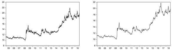
Source: Bloomberg
Figure 2 (Left) Spot exchange rate MXN per 1 USD,

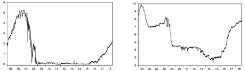
Source: Bloomberg.
Figure 4 (Left) U.S. Treasury Bill yields for 1 month in percentage points, i us,t . (Right) Mexican 28-day CETE in percentage points, i mex,t . Weekly averages of daily data.
LOIS for the U.S. banking system, LOIS us,t , is computed as the weekly average of the difference between the daily 3-month LIBOR in USD and the Overnight Index Swap. The variable LOIS eur,t stands for LOIS for Europe. This is obtained by taking the weekly average of the daily difference between the 3-month Euribor in Euros and the Overnight Index Swap, both published on the Euro Overnight Index Average (EONIA) website. Behaviour of these two measures of funding liquidity shown in Figure 5 is stable, up to the summer of 2007. In particular, LOIS us,t (left) displays several “hump-shape” of financial distress. In 2011 associated with sovereign debt problems in southern Europe. In 2016 associated, possibly to marked changes in regulation (see Du et al., 2018), the “Brexit” Referendum, and sharp volatility observed in markets, mainly reflecting a sharp decline in stock prices. LOIS eur,t (right) also displays several “hump-shaped”. None, however, after those associated with the European sovereign debt
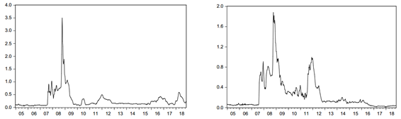
Source: Bloomberg
Figure 5 (Left) Libor-OIS spread in percentage points, LOIS us,t . (Right) Euribor-EONIA rate spread in percentage points, LOIS eur,t . Weekly averages of daily data.
It is worth noting that there is evidence to treat all variables as I(1). In general, a battery of tests fail to reject the null-hypothesis for the presence of a unit root as Table 1 shows. A borderline case arise for LOIS us,t . In particular, the DF − GLS test proposed by Elliott, Rothenberg, and Stock (1996), shown to possess the highest power, when applied to LOIS us,t only rejects the null- hypothesis at the 1% level.
Table 1 Unit root tests
| Variable | ADF µ | ERS | ERS + | PP µ |
|---|---|---|---|---|
| Φ t | -2.260588 | -1.536808 | -0.921692 | -2.870119* |
| ius,t | -1.423635 | -1.418677 | -0.564666 | -1.036137 |
| imex,t | -2.798172 | -1.310672 | -0.906296 | -1.247117 |
| LOIS us,t | -2.385599 | -2.352037* | -1.211621 | -3.089500* |
| LOISeur,t | -2.227629 | -1.865794 | -1.294154 | -2.666757 |
| 5% Critical Value | -2.866976 | -1.941444 | -1.941444 | -2.866868 |
Columns show test-statistic for the Augmented Dickey-Fuller test with
a mean
Note, however, that if these tests are conducted from the period of the peak of the crisis onwards, from September 2008 to October 2018, all variables are unambiguously I(1) as shown in Table 1. This is fairly direct to explain. LOIS ·,t observations were very stable before the crisis, given that there were no major liquidity strains between 2005 and the summer of 2008. Thus, all variables are treated as I(1) in the rest of the paper.
4 Econometric Model and Estimates
Details on the econometric specification of the VECM are now provided. There are several reasons why this model is a suitable tool for the analysis. First, it allows to analyse I(1) variables, and to test the existence of an equilibrium stationary relationship among them (in this case the CIP). Second, it can be transformed into its “common trends representation”, which allows writing each equation of the system as a linear combination of residuals from the VECM (i.e. a Moving Average form), and testing for the number of variables adjusting towards the CIP. Third, it allows the estimation of Impulse Response Functions (IRFs) through the corresponding orthogonalization of the residuals. Finally, it allows to obtain variance and historical decompositions under appropriate conditions of stationarity of the system.
Let n = 5 and define the n × 1 variable vector:4
Let the vector autoregressive model (VAR) in its vector error-correction form of order p, VECM(p),
where
4.1 Specification
Lag-Length
The first step in specifying the VECM is to choose the number of lags, p, used in estimation. Table 2 displays the Bayesian Information Criterion (BIC), the Hannan-Quinn Criterion (H-Q), and the Lagrange Multiplier Test (LM) for autocorrelation for values of p = 1, ..., 15. From Table 2 it is possible to conclude that p = 11 will imply that residuals are free from autocorrelation, since the LM test fail to reject the null hypothesis of no-autocorrelation at the 5% level. Even though p = 11 may seem large, Kilian and Lütkepohl (2017) document that if the true lag-length parameter is unknown, an over-parameterised VAR may yield more accurate IRFs. They also discuss why the Ljung-Box Q test may be biased when I(1) series are involved, hence it is not reported here. In this paper, over-parametrization should not be a concern, provided the sample size is 722 observations.
The canonical VAR analysis no longer requires the residuals to satisfy Normality and Ho- moskedasticity. On the one hand, Normality is no longer a necessary condition to estimate through Maximum Likelihood, since reliance on Quasi-Maximum Likelihood techniques is enough. On the other hand, Heteroskedasticity is no longer an issue in estimating a VAR according to Juselius (2006).
Table 2 p is the lag-length
| p | Reg | BIC | H-Q | LM(1) | LM(p) |
|---|---|---|---|---|---|
| 15 | 76 | -22.944 | -24.449 | 0.000 | 0.004 |
| 14 | 71 | -23.093 | -24.500 | 0.001 | 0.001 |
| 13 | 66 | -23.206 | -24.514 | 0.000 | 0.000 |
| 12 | 61 | -23.306 | -24.515 | 0.000 | 0.000 |
| 11 | 56 | -23.468 | -24.578 | 0.069* | 0.025 |
| 10 | 51 | -23.541 | -24.552 | 0.000 | 0.000 |
| 9 | 46 | -23.656 | -24.567 | 0.000 | 0.001 |
| 8 | 41 | -23.767 | -24.580 | 0.000 | 0.015 |
| 7 | 36 | -23.861 | -24.574 | 0.000 | 0.000 |
| 6 | 31 | -23.969 | -24.583* | 0.000 | 0.000 |
| 5 | 26 | -24.028 | -24.543 | 0.000 | 0.000 |
| 4 | 21 | -24.067* | -24.483 | 0.000 | 0.000 |
| 3 | 16 | -24.054 | -24.371 | 0.000 | 0.000 |
| 2 | 11 | -23.788 | -24.006 | 0.000 | 0.000 |
| 1 | 6 | -23.294 | -23.413 | 0.000 | 0.000 |
Reg is the number of regressors in each equation of the VAR. BIC is the Bayesian Information Criterion on lag length determination. H-Q is the Hannan and Quinn Criterion. LM(p) is the Lagrange Multiplier Test of autocorrelation of order p, for p = 1, ..., 16. * Is the suggested lag according to each criterion. Estimations were made in Dennis, Hansen, Johansen, and Juselius (2005) CATS 2 in RATS.
Rank Test
One of the appealing features of model (4.1) is that it allows to test whether the equilibrium
relationships predicted by economic theory are satisfied by the data. In
particular, when each of the equations (β
′
X
t−1 )j is I(0),
the long-run relationships are satisfied. This is, a subset of elements of
X
t are cointegrated. Note that j =
1, 2.., r < n. Another appealing
feature of the model (4.1) is
that it allows to impose restrictions on the matrix β.
Moreover, if the number of restrictions in each row
Table 3 n − r is the number of Common Trends
| n − r 0 | r 0 | Trace-Stat | Trace-Stat* | Crit-5% | p - value | p − value∗ | BIC |
|---|---|---|---|---|---|---|---|
| 5 | 0 | 130.13 | 121.06 | 76.81 | 0.000 | 0.000 | |
| 4 | 1 | 70.14 | 61.27 | 53.94 | 0.001 | 0.009 | -9.428 |
| 3 | 2 | 27.00 | 22.10 | 35.07 | 0.293 | 0.592 | -9.414 |
| 2 | 3 | 11.56 | 9.49 | 20.16 | 0.497 | 0.693 | -9.381 |
| 1 | 4 | 3.33 | 2.94 | 9.14 | 0.531 | 0.600 | -9.356 |
r is the cointegrating rank (i.e. the number of cointegrating relations). Trace-Stat is Johansen’s Trace Statistic. Crit 5% is the critical value for the size of 5%. Trace-Stat* is Johansen’s small sample corrected Trace Statistic. The null hypothesis is: cointegrating rank = r0. BIC is the Bayesian Information Criterion.
Table 3 contains the tests for several
possible values of r denoted r0. In this case, Johansen’s Trace Test suggests r
= 2. Estimation of
Inspection of (4.4) reveals that
estimates for the main variables of CIP are similar across cointegration
relationships, hence imposing
Expression (4.5) presents the
cointegrating relationship.7 At
this point it is not possible to interpret the estimates. It is possible,
however, to discuss the stationarity of the cointegrating relationship. Figure 6 presents

Table 4 Unit root tests for the cointegrating relationship
| Variable |
|
|
|
|---|---|---|---|
|
|
-3.16 | -6.08 | |
| Sample Mean of |
0.24 | ||
| 5% Critical Value | -1.94 | -1.94 | -1.96 |
Columns show test-statistic for the Augmented Dickey-Fuller test
4.2 Testing the Theoretical Relationship
Assuming that a Data Generating Process can be modelled by a VECM(p) entails the
a priori conjecture that level relationships among the
elements of
Results displayed in expression (4.5) somewhat satisfy conditions 1 and 2, however, condition 3 is
far from being observed. The VECM(p) allows to test whether 3 can be imposed.
Let
Imposing the restriction set (4.6a)-(4.6d), the following estimates are obtained:
The conducted test to assess whether the restrictions imposed in (4.7) are valid suggest they are
not. Table 5 presents the results of the
test which rejects the null hypothesis of
Table 5 Test for the validity of the Restricted Model versus the unrestricted model
| Test of Restrictions | χ 2 | p − value |
|---|---|---|
| Test set A | 25.169 | 0.000 |
| Test set B | 4.3757 | 0.1122 |
The test for set A assumes a χ2(4) distribution. The test assumes a χ2(2) distribution. Null hypothesis: Restrictions are valid.
Since the aim is to test whether changes in funding liquidity are affecting the
CIP, define the restrictions set B as a subset of A where B is composed only by
(4.6a) and (4.6b). That is, define
As shown in Table 5, the Null Hypothesis
of the restriction set B being valid is not rejected at a 10% level. This means
that there is a stationary equilibrium relationship that includes the funding
liquidity measures and has a mean different from zero. Once the validity of the
relationship is established, a test to determine whether

Table 6 Unit root tests for the cointegrating relationship
| Variable |
|
|
|
|---|---|---|---|
|
|
-3.49 | -7.28 | |
| Sample Mean of |
-0.28 | ||
| 5% Critical Value | -1.94 | -1.94 | -1.96 |
Columns show test-statistic for the Augmented Dickey-Fuller test
4.3 Economics of the Estimation
Expression (4.8) should be interpreted as an equilibrium relationship among the 5 elements of X t . In particular, said expression may be written as
where ν t is a mean zero stationary random variable as implied by Table 6.
The relationship between δ t and LOIS us,t is negative, which can be rationalised as follows: (1) An increase in the LOIS us,t spread signals an increase of the perception of credit risk, thus a decrease in funding liquidity in the U.S. (2) The increase in LOIS us,t will cause δ t to decrease in one of three ways: (a) USD appreciates if there is a flight to quality, diminishing the forward premium Φ t ; or (b) i us,t increases since individuals demand less treasuries due to mature in the short run; or (c) both.
The relationship between δ t and LOIS eur,t is positive since: (1) An increase in LOIS eur,t signals a decrease in funding liquidity in Europe. (2) There is a flight-to-quality to the U.S. assets. This causes: (a) an appreciation of the USD, thus Φ t increases (closer to zero); or (b) i us,t decreases; or (c) both.
Finally the constant term represents the minimum profit investors demand to trade MXN and Mexican Treasuries. It is worth noting that despite the similar nature of changes in funding liquidity conditions, whether these are originated in the U.S. or Europe matters. In particular, the two sources of funding liquidity shocks have opposite sign on δ t .
4.4 Weak Exogeneity and the Common Trends Representation
Weak Exogeneity
A further advantage provided by the model (4.1) is that it allows to test for “weakly exogenous variables”. As defined by Juselius (2006, pp. 193), a variable xj,t ∈ {Xt} is said to be weakly exogenous if it affects other variables in the system Xt while it is not affected by them. This is, if the row j of matrix α contains only zeros. Since α is a n × r matrix, and r = 1 in this paper, then a weak exogeneity test is equivalent to testing for each of the 5 rows of α for being different from zero. To this end, a simple t − test statistic is not suitable since the comparison is made across 5 models. In particular, a Likelihood-Ratio statistic is required. Table 7 displays the weak exogeneity test for the variables in Xt.
Table 7 Weak Exogeneity Test
| r | 5% Crit-val | Φ t | i us,t | i mex,t | LOIS us,t | LOIS eur,t |
|---|---|---|---|---|---|---|
| 1 | 3.841 | 9.674 | 12.984 | 0.093 | 0.038 | 1.889 |
| [0.002] | [0.000] | [0.760] | [0.846] | [0.169] |
LR-Test statistic, χ 2(r), p − values in brackets. Null Hypothesis: The variable is weakly exogenous.
Results from the test allow to conclude that i mex,t , LOIS us,t and LOIS eur,t are weakly ex- ogenous. Note, however, that the p-value for i us,t implies that this variable adjusts towards the cointegrating relationship. There is, however, a plausible rationalisation for this seemingly counter- intuitive result. In particular, note that (4.9) contains LOIS us,t and note that funding liquidity shortages may be strongly related to an increase of demand of the safest asset in the market (i.e. the U.S. treasuries). The latter, in turn, should cause yields to change. A similar argument may apply when the change in funding liquidity conditions is born in Europe. This may explain why within the estimated system, i us,t is not weakly exogenous. The latter is confirmed by the restricted estimation and a test for the validity of the restrictions embedded in α˜, contained in Table 8:
Table 8 Test for the validity of the restricted estimate α˜ versus the unrestricted model
| Test restricted α | χ 2 | p - value |
|---|---|---|
| Test of Restrictions | 5.2608 | 0.1537 |
The test assumes a χ2(3) distribution. Null hypothesis: Restrictions are valid. β is left unrestricted.
The restricted estimate for α in equation (4.10), implies that Φ t and i us,t are the only variables of the system that adjust in response to deviations from the cointegration relationship β ′ X t−1 . Moreover, the estimates imply that it takes slightly more than 3 and 7.5 weeks for deviations from the previous period equilibrium relationship to dissipate for Φ t and i us,t , respectively. This is, suppose there is a stationary one-time shock to δ B , seemingly creating arbitrage opportunities.
Their effect on Φ t will take 3 or 7.5 weeks to dissipate entirely.
Common Trends Representation
The VECM also allows writing (4.1) in its common trends representation or Moving Average (MA) form, as proved in the Granger Representation Theorem. This allows both the estimation of the n − r common trends in the system X t and a very intuitive interpretation. The MA form is written as
where β
⊥ is the orthogonal complement of β, defined as the
(n−r)×r matrix satisfying
β
′
β = 0 and similarly for α
⊥.8 The first
component of equation (4.11)
deserves special attention. In particular, note that the product
The n × n matrix C defined in
(4.12) is known as the
“long-run impact matrix” and it is interpreted in two effect of
c
ij on x
i . Row-wise, the element c
ij means if statistically significant, means the
cumulated effect
For the present model, restricted estimates of the long-run impact matrix yield the following common trend representation.9 Recall that Σ is a full matrix as described in (4.3), Table 9 shows the corresponding correlations.
Table 9 Residual Standard Errors and Cross-Correlations
|
|
|
|
|
|
|
|---|---|---|---|---|---|
| S.E. | 0.355 | 0.166 | 0.186 | 0.0667 | 0.0572 |
|
|
1.000 | ||||
|
|
0.634 | 1.000 | |||
|
|
-0.788 | -0.217 | 1.000 | ||
|
|
-0.877 | -0.403 | 0.561 | 1.000 |
The MA form is the representation of each variable as the sum of the history of
previous shocks. Although correlated, these shocks are useful in explaining
changes in each element of system
In line with the weak exogeneity test, equation (4.13) shows all the stochastic trends have a
non-negligible effect on
For i us,t , equation (4.14) shows its non weakly exogenous status. In particular, it is affected by shocks on the forward premium
The results of the estimation for i mex,t displayed in (4.15) suggests some de-coupling of the monetary policy for the period. A case for the presence of at least a second stochastic trend could be made easily in order to explain changes in the Mexican Treasury yield. This issue deserves a deeper study, since the correlations between i mex,t and the rest of the variables is not high enough to justify some second-order effect from a different variable in the system. These second-order effects may be present since the reduced form errors ε t are contemporaneously related
Finally, the MA forms of LOIS us,t and LOIS eur,t in (4.16) and (4.17) show these variables behaving as two weakly exogenous elements, with a high correlation among them
So far, evidence suggests unambiguous support for the relevance of both LOIS us,t and LOIS eur,t in explaining the behaviour of the variables that define δ t . The previous analysis comes a long way in separating effects from each shock into the behaviour of each element of X t . There is a shortcoming,however, and that is related to the covariance matrix of the reduced form errors, Σ contained in Table 9, not being diagonal. Shocks between LOIS us,t and LOIS eur,t cannot be distinguished clearly. To accomplish this, a structural analysis is undertaken in the next section.
4.5 Structural Analysis
The Structural VECM(p) can be readily derived from expressions (4.1) or (4.11). In order to relate the reduced-form errors vector ε t to the “structural” errors vector u t , a Cholesky decomposition is used. This identification strategy relies on the assumption of some causal direction among the variables. Thus, it is assumed that i us,t is independent from the rest of the variables in X t and affects LOIS us,t . In turn, LOIS eur,t is affected by shocks to LOIS us,t . Also, i mex,t is subject to changes in all non-domestic variables. Finally, Φ t responds to shocks to all previous variables. The selected order obeys the economic logic behind the variables in the system. That is, structurally, the i us,t follows its own shocks; the banking system of the U.S. is larger than the European one, however interconnected; the European banking sector is independent of the structural shocks to i mex,t , given that Mexico is a small open economy.10
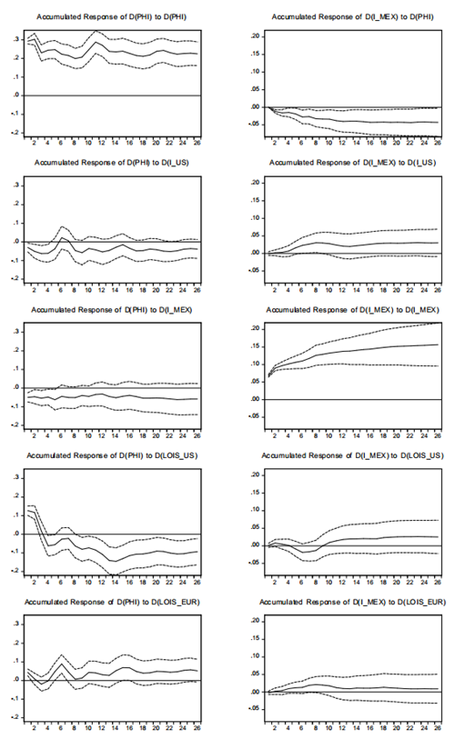
Impulse Response Analysis
The model VECM(11) in (4.1) is used to estimate the IRFs, imposing the identified restriction set (4.8). The responses of both Φ t and i mex,t are displayed in Figure 8. An increase in i mex,t yields a negative response of Φ t , reflecting an MXN appreciation. Also, more stringent funding liquidity conditions given by increases in either LOIS us,t or LOIS eur,t yield a positive response of Φ t . This is, an appreciation of the USD. The right column shows that increases in Φ t , given by an appreciation of the MXN, yield a negative response of i mex,t . Moreover, increases in either i us,t or LOIS eur,t imply an increase in i mex,t . Note that this is the expected monetary policy reaction to more stringent funding conditions, in a broad sense.
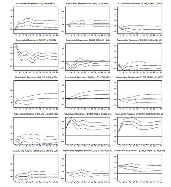
The response of the rest of the variables to the shocks is shown in Figure 9. As suggested by the weak exogeneity analysis, i us,t responds positively to increases in Φ t and to no other shock. More- over, LOIS us,t responds negatively to shocks to i us,t and LOIS eur,t . Finally, LOIS eur,t responds negatively to increases in both Φ t and i us,t , while responding positively to shocks to LOIS us,t .
Forecast Variance Decomposition Analysis
A forecast variance decomposition analysis is undertaken to complete the analysis of the aver- age effect of shocks to the variables. Having established that funding liquidity shocks have a role in explaining deviations form the CIP, the aim is to quantify the relative importance of changes in LOIS us,t and LOIS eur,t . To this end, a VAR model in levels based on the VECM(11) is esti- mated. As discussed by Kilian and Lütkepohl (2017), the analysis may well be carried out on the VECM(11) even though all variables contained in X t are I(1). This, however, may entail some loss of information since the model is expressed in differences.
Estimation was carried out in EViews 10.
Figure 8 Impulse Response Functions and ± 2 Standard Errors computed by Monte Carlo Simulations.
Estimation was carried out in EViews 10.
Figure 9 Impulse Response Functions and ± 2 Standard Errors computed by Monte Carlo Simulations.
The estimated VAR model in levels is given by
where X
t = (LOIS
us,t
, LOIS
eur,t
, δ
t )′, δ
t is defined in (2.4),
Results from the forecast error variance decomposition for
Table 10 Forecast Error Variance Decomposition
| Horizon | S.E. | δ t | LOIS us,t | LOISeur,t |
|---|---|---|---|---|
| 1 | 0.364533 | 75.46490 | 21.27821 | 3.256888 |
| (2.92715) | (2.67605) | (1.12950) | ||
| 5 | 0.593349 | 76.85711 | 20.53360 | 2.609291 |
| (2.82405) | (2.58550) | (1.37738) | ||
| 10 | 0.674929 | 64.28828 | 29.05565 | 6.656070 |
| (5.02050) | (4.38689) | (3.39428) | ||
| 15 | 0.775626 | 53.96670 | 38.88517 | 7.148130 |
| (5.53852) | (5.29684) | (4.13493) | ||
| 25 | 0.824555 | 48.13689 | 41.03941 | 10.82371 |
| (6.10063) | (6.17755) | (6.31722) | ||
| 52 | 0.862945 | 44.93074 | 40.46760 | 14.60166 |
| (6.25840) | (6.83538) | (8.61251) |
S.E. stands for the forecast error at each horizon. The labelled columns labelled with the elements of X t are the percentage of the forecast variance attributed to each variable. Standard Errors computed by 104 Monte Carlo Simulations are shown within brackets. Estimation was carried out in EViews 10.
Interestingly, the relative importance of LOIS us,t is statistically the same as that of δ t in ex- plaining the forecast error variance of δ t after 15 weeks. The latter may be rationalised by, first, noting that the U.S. banking sector is the largest in the world and, second, the analysis of the CIP involves the USD, the currency in which LOIS us,t is determined.
A further result worth of attention is that, however small when compared with LOISus,t, changes in LOISeur,t are important in explaining deviations from the CIP. Indeed, in a horizon of 52 weeks, 14.6% of the forecasts error variance may be attributed to this funding liquidity measure. Thus evidence supports that, notwithstanding the apparent weak relationship that may exist between the USD-MXN market and European financial markets, there is a non-negligible link.
Historical Decomposition Analysis
Up to this stage, the structural analysis suggests that on average, changes in funding liquidity conditions are relevant to determine deviations from CIP. The analysed period is characterised by a sequence of financial events, not all taking place simultaneously. Hence, an Historical Decomposition Analysis may shed light on the relative importance of each measure of funding liquidity at each date. Figure 10 displays the results. In particular, the solid line is the relative importance of each variable on the behaviour of δ t while the shade corresponds to de-mean δ t itself.
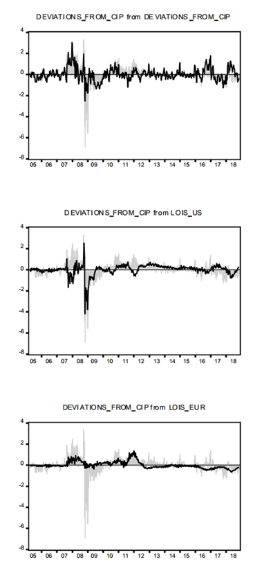
Shaded area corresponds to δ t , solid line corresponds to the relative importance of each variable explaining δ t . Estimation was carried out in EViews 10.
Figure 10 Historical Decomposition of δ t computed by Monte Carlo Simulations.
Some conclusions emerge. Prior to the onset of the financial crisis in summer 2007, most of the dynamics of δ t were explained by itself (i.e. changes in Φ t , i us,t , and i mex,t ). After August 2007, the funding liquidity measures are able to explain several episodes of stark deviations from CIP. In particular LOIS us,t is able to account for the observed large deviations from early 2008 to mid 2009, including of course those registered in the fourth quarter of 2008 when Lehman failed, AIG was bailed-out, and TARP was approved by the U.S.’ Congress. It then explains a large share of δ t from mid 2010 to mid 2011. Finally, beginning in 2012, possibly related to new regulation concerning funding of commercial banks, the funding liquidity measure re-gained importance.
The role of LOIS eur,t is reflected mainly in four episodes. First, from mid 2007 to mid 2008, a period where, as documented by Ivashina et al. (2015), European banks experienced marked USD liquidity constraints. Second, from mid 2010 to early 2011, when several southern European economies were on the brink of entering into a sovereign debt crisis. Third, throughout 2011 when the sovereign debt crisis was at its peak, particularly in Greece. The role of LOIS eur,t started to diminish after the European Central Bank (ECB) stated that “Within our mandate, the ECB is ready to do whatever it takes to preserve the euro.” in mid 2012.12 Finally, towards the end of the sample in 2018, this funding liquidity measure is able to account for deviations from the CIP.
5 Concluding Remarks
In this paper, econometric evidence is presented to support the hypothesis that
funding liquidity constraints have a significant role in explaining deviations from
CIP relating the USD-MXN. Results show that the LOIS spread in USD is positively
related to deviations from CIP whereas the LOIS spread in EUR is negatively related,
underscoring that the source of the shock matters. Moreover, it is found that both
funding liquidity measures are able to explain the forecast error variance of
deviations from CIP. Interestingly, LOIS in USD accounts for a similar share of said
variance than deviations from CIP after 15 periods. An historical decomposition
analysis suggests that both LOIS in USD and EUR are able to account for both
positive and negative deviations from CIP. The analysis suggests that the the
apparent arbitrage opportunities do not exist once funding liquidity conditions are
included. This is, there should be no deviations from the CIP once funding liquidity
conditions are considered. From the policy perspective, this paper underlies the
relevance of funding liquidity measures when assessing whether the USD-MXN foreign
exchange is functioning efficiently. There are some caveats in the analysis to
consider. First, the borderline conclusion of the funding liquidity measures being
I(1) should be present before making further conclusions.
Second, many market participants are not able to fund their liquidity at LIBOR or
OIS rates, but at higher ones. Future work should aim to find a funding liquidity
measure for non-prime borrowers. Further research should focus on testing different
models that account for the borderline stationarity of the


