1. Introduction

Over the past decades, it has been observed that there has been a growth in interest in microwave sensors operating in the near field regime. These sensors are based on a printed circuit technology, are very compact, extremely cheap and possess higher sensitivity compared to volumetric counterparts. The passive elements usually are planar microwave resonators with a high-quality factor. Conventional electronics measures a shift in their resonant curves caused by a complex permittivity of a sample under test.

Since the devices are very universal, they are used for the characterization of a wide spectrum of materials, such as solids, liquids, biological samples, vapors (^{Alahnomi et al., 2021}). The most complete data processing method for this technology is known as dielectric (or impedance) spectroscopy that measures the dielectric properties of a medium as a function of an external field frequency (^{Kremer & Schönhals, 2003}).

Less attention was paid, however, to active microwave sensors, in particular to the oscillators where a resonant element is a part of a positive feedback loop. In this case a microwave resonator modulates the parameters of an auto-oscillation

frequency, when interacting with a sample. This technique is a microwave analogue of the intracavity laser spectroscopy (^{Baev et al., 1999}), including the mixed laser-microwave double resonance spectrometry (^{Jones, 1977}), and is implemented in the millimeter-wave range on the basis of an Ortotron oscillator (^{Rusin & Bogomolov, 1969}).

2. Steel production

The diagram of the delay line ring oscillator is shown in Figure 1 The principal element of the magnonic oscillator was a 5 mm x 2 mm rectangular ferromagnetic sample, composed of a 7.3 μm thick yttrium iron garnet (YIG) film grown on a 0.5 mm thick gadolinium gallium garnet (GGG) substrate. The YIG/GGG element was saturated in a bias magnetic field (H0) along the Y axis. The YIG/GGG structure was placed on a printed electrode circuit fabricated on a composite ceramic substrate.

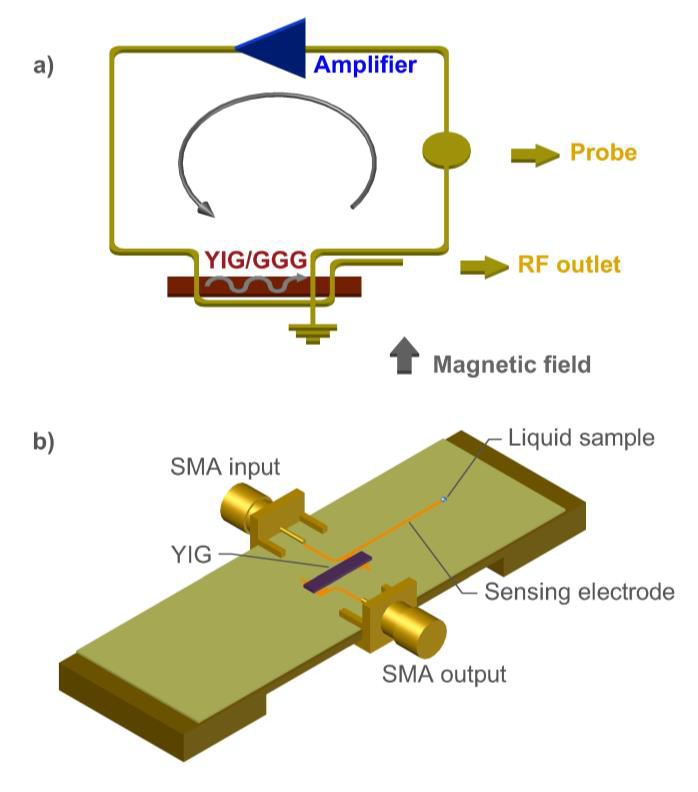
Figure 1 a) A schematic of the microwave ring oscillator based on MSSW delay line; b) implementation of the microstrip line structure with the YIG/GGG delay line on a ceramic substrate (ε = 9, Rodgers Corp.). 

The printed circuit contains two transducers with periodic electrode structure, microstrip line stub (sensing electrode), as well as input and output ports. The geometry in Figure 1 provides excitation and propagation of magnetostatic surface wave (MSSW) in YIG film along the X direction (Fig. 1) (^{Prabhakar & Stancil, 2009}).

The shorted periodic electrodes are shown in Figure 2. This structure is used for efficient excitation and detection of MSSWs. The system operates as a delay line whose insertion loss was approximately 10dBcm within 1-3 GHz frequency range. The delay line was connected to input and output ports of a solid-state amplifier. The circuit provided the Barkhausen criterion for the oscillation within the frequency range from 0.9 to 1.5 GHz. It was possible to tune the oscillator frequency by varying H0. In order to measure the oscillation frequency, we used an additional antenna coupled the feedback loop. The output signal of the oscillator was approximately 10 mW. At the bias field of H0= 200 Oe the oscillation frequency was ≈1.3 GHz, and typical wavelength of MSSW, determined by the periodic electrode, was ~600 μm. Using a spectrum analyzer RSA306B the linewidth of this signal was measured to be about of 0.6 KHz. The details on similar magnonic oscillators are described in (^{Bankowski et al., 2015}; ^{Castéra & Hartemann, 1985}; ^{Ishak, 1983}).

Figure 2 A zoomed view of the periodic electrode structure with shorted end. 

The operational principle of the system is based on a shift in the oscillator frequency due to the phase perturbations in the sensing electrode caused by a liquid sample (Figure 1b) that induces changes in the complex relative permittivity ε=ε'-jε'', in the vicinity of the opened electrode end. Here, ε'=Re(ε)/ε0 and ε''=Im(ε)/ε0, and ε0 is the vacuum permittivity. Note, with a certain approach ε'' can be expressed through the conductivity of a material (σ) as ε''=σ/(ω0ε0), or the electric loss tangent ε''=ε'tan⁡(δ). The peculiarity of the sensor is that both the ε' and the sample losses ε'' cause a down shift of the oscillator frequency. They induce the phase shift in the structure composed of the sensing electrode connected to the periodic transducer, in the point “A” in Figure 2. This structure acts as a microstrip line resonator that possesses parallel resonance at a specific frequency. A detailed technical description of the sensor is presented in the Appendix.

3. Experimental methodology and formation of droplets

The basic aim of this work was the evaluation of capability of the system to discriminate liquids with different percentage of salt concentrations and organic inclusions from their nano-liter volumes. If the water contains salt, the real part of permittivity is slightly reduced, but the imaginary part is increased significantly making the water even more dominating.

It should be noted that in most of the works the aqueous solutions have been characterized by the dielectric spectroscopy (a wide range frequency sweeping) of large volumes of the samples. In this case, there are no technical problems to substitute one sample by another one. However, in the case of nano-volume sessile droplets it is difficult technically to provide a calibrated volume and exact position of the droplet each time when a liquid sample is replaced by another. After experimental analysis of several deposition and detection techniques, including microfluidic method as well as deposition of a droplet matrix, we found that more effective method is a cycle of periodic deposition - evaporation of a droplets formed at the sensing electrode because of the accumulative effect and strong dependence of a droplet evaporation time on the concentration of salts and inclusions.

The deposition of nano-litter sessile droplets on the sensing resonator was a completely automatized process, controlled by LabView data acquisition platform. We used a Hamilton 7000 Series 0.5 microliter syringe. The syringe was fixed in Thorlabs optical translation stages integrated with linear actuators controlled by a PC. The droplets were formed at the opened end of the sensing resonator where the electric field is maximum, as shown in Figure 3. The droplets formation system was designed to deposit a series of droplets of constant volume of 30 nano-liters, at a specific time interval between them, determined by an evaporation time of a single droplet. Figure 4 illustrates the steps of the droplet deposition.

Figure 3 The sensing electrode with a sessile droplet. 

Figure 4 The droplet formation steps: down displacement of the syringe from position 1 to position 2; formation of the sessile droplet 3; up displacement of the syringe from the position 3 to the position 4. Steps 1 - 4 are repeated after the droplet. 

4. Experimental results

4.1. Water salinity

Figure 5 shows typical waveforms at the periodic deposition - evaporation of H ₂ O+NaCl sessile droplets with different concentrations of NaCl. The aqueous solutions for this experiment were prepared from deionized water (di-H ₂ O). The diagrams show the oscillator down frequency shift vs the droplets evaporation time. The oscillator frequency was measured by a frequency counter integrated into LabView® platform. As seen in Figure 5, the droplet deposition causes 300 KHz frequency down shift (∆f) of the oscillator. Considering that the oscillation line bandwidth is of 0.6 kHz, the signal is composed from ≈500 resolved points over the ∆f range. Note, in Figure 5 the curves for different concentrations were shifted on the frequency axis from zero level just to avoid their overlapping. The experiment shows that the evaporation time, accumulated by M=6 depositions, increases by approximately 2 times, as the NaCl concentration increases from 0 to the saturated value.

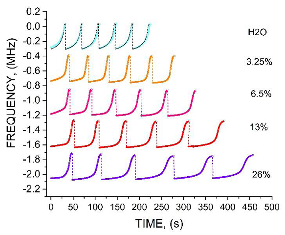
Figure 5 The droplet formation steps: down displacement of the syringe from position 1 to position 2; formation of the sessile droplet 3; up displacement of the syringe from the position 3 to the position 4. Steps 1 - 4 are repeated after the droplet. 

The details of evaporation dynamics of the droplet are presented in Figure 6 that shows five specific parameters, which characterize the evaporation process. First, it is the droplet evaporation time W (as seen in Figure 5 W depends on M), then, maximal frequency shift FS, and three stages of the evaporation response with the specific slopes τ1, τ2, and τ3. Therefore, the method measures the four-component vector.

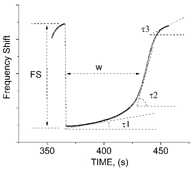
Figure 6 The last period of the droplet evaporation for the case shown in Fig. 5 for 26% concentration. The curve shows the evaporation time W, maximal frequency shift FS, as well as three stages of the evaporation response with the specific slopes τ1, τ2, and τ3. 

Figure 7 shows the evaporation time of the droplets with different NaCl concentrations, accumulated over 6 evaporation-deposition periods. The data was extracted from the experiment like in Figure 5. Figure 8 shows that 15 evaporation periods allow one to discriminate the accumulated difference between the di-water and the water at the salinity of S = 0.5 psu (1psu ≈ 1ppt, parts per thousand, or 0.05% of NaCl concentration).

Figure 7 The evaporation time accumulated over M = 6 periods vs NaCl concentration. 

Figure 8 Evaporation for di-H2O (the curve 1) and the solution with 0.05% of NaCl (2). 

4.2. Total dissolved and suspended solids

For characterization of purity of water also there are two parameters of interest: total dissolved and total suspended solids. Total dissolved solids (TDS) is an aggregate measure of charged and uncharged inorganic and organic compounds completely dissolved in water, including both volatile and non-volatile. Volatile solids are ones that can easily go from a solid to a liquid state. Examples of non-volatile substances include salts and sugars. The two principal methods of measuring TDS are the gravimetric analysis and conductometric methods. Gravimetric methods (GM) are the most accurate and involve evaporating the liquid solvent and measuring the mass of residues left. GM, however, are time consuming if involve large volumes of aqueous solution. The conductometric methods (CM) are fast, but they are not sensitive to uncharged compounds or low-charged ions like motor oil, gasoline, many pharmaceuticals, and pesticides. It should be noted, both GM and CM are not suitable for the detection of the so-called PFAS molecules, which are made up of a chain of linked carbon and fluorine atoms. This analysis can be provided only in specialized laboratories by using sophisticated liquid chromatography combined with mass spectrometry. Total suspended solids (TSS) are undissolved suspended inclusions in water. The basic laboratory method for TSS detection is their extraction by filtering the sample. Also, light scattering is used in portable devices.

The advantage of microwave methods is that they detect changes in dielectric constant caused both by conductivity and by molecular polarization, i.e. microwave probes are capable of detecting uncharged particles. Here we present the results revealing how our microwave sensor can be used for TDS/TSS detection, by analyzing aqueous samples with organic suspension. As seen in Figure 9, sea water sample induces a monotonic decrease in the amplitude of the frequency shift over the deposition-evaporation set. This decrease in FS is characterized by the slope angle β in Figure 9. We attribute this behavior to a thin layer of TSS growing on the sensing electrode after each evaporation. The monotonic decrease of FS takes place because of the increase of the vertical distance between the droplet and the sensing electrode plane, as the TSS layer thickness increases. In contrast, as seen in Figure 5, the sensing electrode practically does not “feel” the NaCl microcrystals left on its surface after the evaporation. This takes place because in our case the NaCl micro crystals are rapidly dissolved at each deposition of the droplet. Consequently, NaCl concentration and evaporation time of each subsequent droplet increases (W depends on M in Figure 5). The clear difference between di-H ₂ O, salted water and sea water is presented in Figure 10.

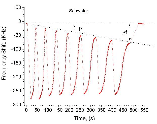
Figure 9 A peculiarity of sea water droplet evaporation: a) the fact that each subsequent deposition increases W indicates that the sample has dissolved salts, b) the decrease of the initial level of FS takes place due to TSS. Note, FS returns to the initial zero level after the last evaporation of sea water sample because the sensing electrode surface was cleaned. 

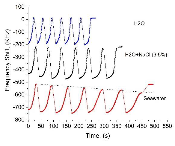
Figure 10 The effects of the salinity (the curve H2O+NaCl), and the salinity combined with TSS (seawater). The data indicate that sea water contains more types of dissolved salts compared to NaCl solution, because, as seen in the figure, the accumulated evaporation time of sea water exceeds the accumulated evaporation time of NaCl solution. 

Figure 11 shows similarity between sea water and urine sample that includes organic suspension. It is clearly seen in Figure 10, and Figure 11 that the width W of each subsequent evaporation profile in the curves with organic compounds increases, i.e. W is a function of M, like in Figure 5. It means that the samples contain dissolved salts. Their concentration can be evaluated from the dependence W(M), and the difference M (W_H2O - W_H2O+N_aCl). Therefore, we expect that the sensor is capable of discriminating TSS from dissolved salts.

Figure 11 The effects of salinity combined with TSS for urine and seawater. 

5. Discussion

For the comparison, in Figure 12 we present the measurement of FS for different liquids by using a thin-wall Teflon capillary tube, at 0.2 mm inner diameter, attached along the Y direction to the substrate shown in Figure 1b, close to the sensing electrode end. This configuration provides a fixed volume of aqueous solution. Figure 12 shows the oscillator response, as a liquid sample was periodically pumped in and out of the capillary tube. The difference in the frequency shift (∆FS) between di-H ₂ O and the solution with 3.5% concentration of NaCl in Figure 12 is about of 90 kHz, and the (mean absolute deviation of FS) was about of δFS=2 kHz. Hence, the precision of this technique is ≈2%, and the resolution with respect to NaCl concentration is δS=(3.5%)/N=0.077% (or 0.7 psu, in practical salinity units), where N=∆FS/δFS=45 is the number of the resolved levels of FS. Note, in our experiments the sample temperature was not stabilized. For the comparison, the precision of the thermo-controlled volumetric resonant cavity method for the measurement of ( is δε=0.2-0.3 (or (δε/ε)100≈0.3%), and the error is δS=0.2 psu, or 0.02%, at water salinity S=30-50 psu (^{Gadani et al., 2012}; ^{Lang et al., 2015}).

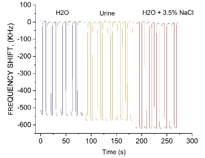
Figure 12 Frequency shift of the oscillator due to microfluidic flow of di-water, urine, and 3.5% NaCl solution through a thin-wall Teflon capillary tube attached to the sensing electrode end. 

On the other hand the difference in the accumulated evaporation time (W), due to M=6 depositions, between the distilled water and the solution with 3.25% NaCl concentration in Figure 5 is about of M(WH2O - WH2O+NaCl) = 55s, and the mean absolute deviation of W was about of δW=1s. Hence, in this case one can obtain N≈50 resolved values of W within the salinity percentage 0-3.25%, i.e., the resolution of the evaporation method with respect to NaCl concentrations is δS≈(3.25%)/N=0.06% (or 0.6 psu), that is close to our microfluidic capillary tube method. Also, the evaporation dynamics gives four additional parameters (τ1,τ2,τ3) to be involved into the analysis of a sample, as seen in Figure 5. Moreover, the resolution of the periodic deposition-evaporation technique can be increased by increasing the number of the cycles M. It is demonstrated in Figure 8, where the accumulated evaporation time of 15 cycles allowed us to measure a difference between di-H2O and the water with the salinity S=0.5 psu (or 0.05% of NaCl concentration). In this case, the resolution of the method, δS≈0.03 psu, approximates to the resolution δS=0.1-0.01 psu of portable salinity meters, based in the measurements of the conductivity.

Here we do not discuss the accuracy required for the determination of the absolute values since the device has to be carefully calibrated. It is especially important when measuring TSS. Also, we suppose that the device can be calibrated to measure TDS. For the experiments shown in Figure 11 we used NaCl solution at the concentration that approaches to the salinity of the sea water sample. In addition to the discussed TSS effect, the observed difference in the accumulated evaporation time between di-H2O, NaCl solution, and sea water allows one to extract the information about TDD in sea water, by deducting the accumulated evaporation time from H2O+NaCl and sea water samples.

6. Conclusions

In this work we described the microwave intracavity sensor for the characterization of aqueous solutions of nano-liter sessile droplets, deposited on the microstrip line electrode. It operates at GHz frequency and is based on tunable magnonic delay line oscillator. The samples were characterized by using their evaporation dynamics, by measuring their dielectric constants. The presented (proof of concept) experiments have shown that the sensor can detect the salinity of water with the required precision and resolution. The advantage of the sensor is the possibility of measuring the parameters such as S, TSS and TDS, simultaneously.

References

Alahnomi, R. A., Zakaria, Z., Yussof, Z. M., Althuwayb, A. A., Alhegazi, A., Alsariera, H., & Rahman, N. A. (2021). Review of Recent Microwave Planar Resonator-Based Sensors: Techniques of Complex Permittivity Extraction, Applications, Open Challenges and Future Research Directions. Sensors, 21, 2267. https://doi.org/10.3390/s21072267 [ Links ]
Baev, V. M., Latz, T., & Tochek, P.E. (1999). Laser Intracavity Absorption Spectroscopy. Applied Physics B 69(3):171-202. https://doi.org/10.1007/s003400050793 [ Links ]
Bankowski, E., Meitzler, T., Khymyn, R., Tiberkevich, V.S., Slavin, A. N., & Tang, H. X. (2015). Magnonic crystal as a delay line for low-noise auto-oscillators. Applied Physics Letters, 107. p. 122409. https://doi.org/10.1063/1.4931758 [ Links ]
Castéra, J. P., & Hartemann, P. (1985). Magnetostatic wave resonators and oscillators. Circuits Systems and Signal Process. V. 4. 181-200. https://doi.org/10.1007/BF01600079 [ Links ]
Gadani, D.H., Rana, V.A., Bhatnagar, S.P., Prajapati, A. N., & Vyas, A. D. (2012). Effect of salinity on the dielectric properties of water. Indian Journal of Pure & Applied Physics. Vol. 50, pp. 405-410. http://nopr.niscpr.res.in/handle/123456789/14183Links ]
Ishak, W. (1983). 4-20 GHz Magnetostatic wave delay-line oscillator. Electronics Letters. V. 19 No. 22. P.930-931. https://doi.org/10.1049/el:19830635 [ Links ]
Jones, H. (1977). Wide-Band Intracavity Microwave Cells for Laser-Microwave Double Resonance Spectrometry. Appl. Phys. 14. 169 - 173. https://doi.org/10.1007/BF00883085 [ Links ]
Kremer F., & Schönhals A. (2003). Broadband Dielectric Spectroscopy. Springer-Verlag Berlin Heidelberg. ISBN 978-3-642-56120-7 https://doi.org/10.1007/978-3-642-56120-7 [ Links ]
Lang, R., Zhou, Y., Utku, C., & Le Vine, D. (2015). Accurate measurements of the dielectric constant of seawater at L band. Radio Sci., 51. 2-24. https://doi.org/10.1002/2015RS005776 [ Links ]
Li, M. H., Lu, R., Manzaneque, T., & Gong, S. (2020). Low Phase Noise RF Oscillators Based on Thin-Film Lithium Niobate Acoustic Delay Lines. Journ. of Micromechanical Systems , V. 29 , NO. 2. p.p. 129-131. https://doi.org/10.1109/JMEMS.2019.2961976 [ Links ]
Matatagui, D., Kolokoltsev, O.V., Qureshi, N., Mejía, E.V., & Saniger, J.M. (2015). A novel ultra-high frequency humidity sensor based on a magnetostatic spin wave oscillator. Sensors and Actuators B-chemical, 210, 297-301. https://doi.org/10.1016/j.snb.2014.12.118 [ Links ]
Rusin, F. S. & Bogomolov, G. D. (1969). Orotron - An electronic oscillator with an open resonator and reflecting grating, Proceedings of the IEEE, vol. 57, no. 4, pp. 720-722. https://doi.org/10.1109/PROC.1969.7049 [ Links ]
Sefiane, K., Tadrist, L., & Douglas, M. (2003). Experimental study of evaporating water-ethanol mixture sessile drop: influence of concentration. International Journal of Heat and Mass Transfer, 46, 4527-45347. https://doi.org/10.1016/S0017-9310(03)00267-9 [ Links ]
Somaraju, R., & Trumpf, J. (2006). Frequency, Temperature and Salinity Variation of the Permittivity of Seawater. IEEE Transactions on Antennas and Propagation, vol. 54, no. 11, pp. 3441-3448. https://doi.org/10.1109/TAP.2006.884290 [ Links ]
Soulié, V., Karpitschka, S., Lequien, F., Prene, P., Zemb, T., Moehwalda, H., and Hans, R. (2015). The evaporation behavior of sessile droplets from aqueous saline solutions. Phys.Chem.Chem.Phys. 17. p.p. 22296- 22303. http://dx.doi.org/10.1039/C5CP02444G [ Links ]
Prabhakar, A., & Stancil, D. D. (2009). Spin Waves: Theory and Applications. Springer Science & Business Media. 348 p. ISBN 978-0-387-77865-5 https://doi.org/10.1007/978-0-387-77865-5 [ Links ]
Zang, D., Tarafdar S., Tarasevich Y.Y., Choudhury, M.D., & Dutta, T. (2019). Evaporation of a Droplet: From physics to applications. Physics Reports 804. P.p.1-56. https://doi.org/10.1016/j.physrep.2019.01.008 [ Links ]
Peer Review under the responsibility of Universidad Nacional Autónoma de México.
Funding
The authors received no specific funding for this work.
Appendix
The peculiarity of the design of the sensing electrode system is the following. The sensing electrode alone was designed as an opened end microstrip line resonator with a λ/2 resonance at ωS=2.4 GHz, and λ/4 resonance at ω1=1.3GHz. Figure 13 shows these resonances simulated with the help of the “Microwave Studio (MWS)” software. Below the frequency ω1 (Figure 13) the microstrip line possesses a capacitive impedance XC=-j/ωC, where C is capacitance of the microstrip line. In turn, the periodic electrode structure has an inductive impedance XL=jωL. When they are connected, at point A in Fig. 1, they form a parallel resonant circuit that has a resonance ωp, somewhat below of ω1. The optimal sensitivity of the sensor takes place when the oscillator frequency ω0 is set to be ω0<ωP. The advantage of the magnonic oscillator is that this can be done by adjusting H0.
Figure 13 The input impedance Z11 of the sensing electrode alone (disconnected from the periodic structure).
The structure, composed of the opened-end sensing electrode connected to the shorted periodic transducer and a liquid sample, shown in Figure 1b, was also simulated by the “Microwave Studio”. Figure 14 shows the reflection parameter S11 calculated at the input port, at different values of the real permittivity (ε') and conductivity (σ) of the sample. In the simulations we used the ranges of ε' and σ, which correspond to different salinity of water (from 5 psu to moderate salinity of 30 psu, ref. 10). Although in real salted water σ increases and ε decreases, as the water salinity increases, here, in the simulations we used these parameters as independent ones, to reveal how ε' and σ affect the S11 resonance curve. As seen in Figure 14, the conductivity σ plays the dominant role in the perturbation of the S11 resonance curve.
Figure 14 The calculated reflection parameter S11 of the resonant electrode structure shown in Figure 1b, with a liquid sample: a) the sample conductivity σ changes from 0.01 to 3 S/m, at the fixed ε' = 80; b) ε' of the sample changes from 70 to 80, at the fixed σ = 0.01 S/m. Note, the resonance curve of the structure is down shifted, as ε' increases from 70 to 80.
The resonant circuit model
Figure 15 shows a simplified model of the resonant circuit shown in Figure 1b built with the help of the “Microwave Office (MWO)” software. The reflection (S11) and transmission (S21) parameters of the model in Figure 15a are presented in Figure 16. Note, the equivalent circuit Figure 15b gives a similar result.
Figure 15 a) The microstrip line MWO model of the 23 mm long sensing electrode (STUB) connected to the periodic transducer (TL7). The microstrip line “SAMPLE” simulates a sessile droplet; b) The equivalent circuit of the structure shown in Figure 1b, at a frequency ( < (p. Here, ML is the feeder microstrip line, L is the inductance of the periodic electrode, C is the capacitance of the sensing electrode, R is the loss factor.
Figure 16. The S11 and S21 resonances of the opened-end sensing electrode connected to the shorted periodic transducer, calculated for the MWO model in Figure 5a, for the case when the dielectric parameters of the microstrip line “SAMPLE” are the same as those of the sensing electrode (i.e. there is no aqueous solution). The resonances correspond to the parallel RCL circuit equivalent model.
Figure 16 The S11 and S21 resonances of the opened-end sensing electrode connected to the shorted periodic transducer, calculated for the MWO model in Figure 5a, for the case when the dielectric parameters of the microstrip line “SAMPLE” are the same as those of the sensing electrode (i.e. there is no aqueous solution). The resonances correspond to the parallel RCL circuit equivalent model.
The operation principle of the sensor can be explained with the help of MWO model presented in Figure 17. Figure 18 shows the frequency dependence of the phase shift in the delay line oscillator loop vs the dielectric parameters of the microstrip line segment “SAMPLE” representing the aqueous solution. The phase curves in Figure 18 were calculated from the scattering parameter S56 of the ports in Figure 18. For visual clarity of the results presented in Figure 18, in this model we used the dispersion-less 100 ns delay line from the MWO library. It should be noted that real MSW delay line is dispersive element and has ≈200 ns delay.
Figure 17 The model of the oscillator was analyzed by Microwave Office software. Here, the basic microstrip line structure was built on the loss-less substrate with the dielectric permittivity of ε = 9, and the sample is represented by a 0.5 mm-short microstrip line on the substrate with variable ε' and losses (tanδ). The layout includes a sample, the sensing electrode structure, the 6 dB gain amplifier, and the delay line. It should be noted that the amplifier gain is below those required for auto-oscillation. The elements “TL12, STUB, and SAMPLE” represent the resonator with parallel resonance at ωP
The phase curve P1 in Fig. 18 shows of the oscillator loop without the sample. Then, one can see that in the presence of the “sample” with ε'=80 and ε''0 the curve P1 is down shifted to the phase curve P2. Now, let us suppose that the sample is 3.5% of NaCl dissolved in distilled water. This concentration decreases ε' from 80 to 70 and (// increases from 5 to ( 100 [x, x]. In the loss-less case, ε'=70 and at ε''0, the phase curve P2 in Fig. 18 is up shifted to the curve P3. However, “switching on” the losses ε''=100 leads to the broadening of the phase resonance shown by the curve P4 (i.e., at ε' = 70 the curve P3 for ε''0 is transformed to the curve P4 for ε''=100).
Figure 18 The phase-frequency ((f) characteristics of the delay line oscillator. The curve P1 shows ((f) without a sample, the curve P2 simulates a “sample” at ε' = 80 and ε'' ≈ 0, P3 shows the case ε' = 70 and ε'' ≈ 0, and P4 shows the case ε' = 70 and ε'' ≈ 100 . The curves S11 and S21 are the scattering parameters of the passive resonator.
As we mentioned above, the oscillator frequency ω0 must be detuned a few MHz below from the resonance ωP of the parallel resonant electrode structure, by adjusting H0. The resonance ωP is shown in Figure 18 (only as the reference) by the curves S11, S21 calculated from the model in Figure 15. The operation frequency range of the oscillator is shown in Figure 18 by the region designated as “ f0”. Figure 19 shows the phase curves P3-P4 within this region. As seen in the figure, although the decrease of ε' from 80 to 70 up-shifts the phase curve waveform, the broadening of the phase curve due to increased losses (or the sample conductivity) finally leads to the down frequency shift of the phase curve. The arrow in Figure 19 (pointing from the frequency f0) shows the resulting shift of the oscillator frequency to a lower frequency that provides the Barkhausen criterion for the oscillation. Therefore, even though the salinity (or conductivity) of the aqueous solution decreases ε', nevertheless the oscillator frequency decreases because of very strong increase of ε''.
Figure 19 MWO simulations of the modulus and the phase of the transmission coefficient S21 for the layout shown in Figure 7. The curves 1 and 4 show the case when the real permittivity of the sample is ε' = 80, and tanδ = 0. The curves 2 and 5 show the case when the real permittivity of the sample is ε' = 80, and tanδ = 0.5 (ε'' ≈ 40). The curve 3 shows the transmission parameter S21 of the circuit without both the amplifier and delay line (no feedback, as in Figure 4). The parameter ∆F shows the operation frequency range of the sensor.
Mathematical analysis of the oscillator can be done by the transfer function method. Let us consider the layout in Figure 17 in which the electrode system is substituted by the parallel RLC resonator shown in Figure 14b. The transfer function of the delay line oscillator is (Li et al., 2020)
H=G1-Gh Eq 1
Where: G is the amplifier gain, h=DT, D=ejωτ is the transfer function of the delay line, where τ is the time delay,
T=jRCω1LC-ω2+jωRC Eq 2
is the transfer function of the parallel RLC circuit.
Calculated transfer function H is presented in Figure 19. The simulation was done at the inductance L = 2 nH, and the capacitance C = 7 pF. As seen in the Figure 20, the oscillation frequency acquires 5 MHz down shift when the capacitance was changed from C to C+δC, where δC=0.1pF (δC is induced by a sample), and RLC loss was changed from R 50 to 100 Ohm, respectively.
Figure 20 The function H of the active ring at G ≈ 1 and τd = 100 ns. The curves 1 and 2 show the shift of the oscillation frequency as the capacitance of the RLC circuit increases by 0.1 pF and loss parameter R changes from 50 Ohm and 100 Ohm, respectively. Curve 3 shows the transmission parameter S21 of the RLC filter.
Received: May 19, 2022; Accepted: October 18, 2022; Published: April 30, 2023
*Corresponding author. E-mail address: rodreyes.87@gmail.com (C. Rodríguez-Reyes).
Conflict of interest
The authors have no conflict of interest to declare.
Creative Commons License This is an open-access article distributed under the terms of the Creative Commons Attribution License